Research notes
Solving the multicomponent UVN flash in TVN space
A step-by-step account of stability analysis, entropy maximization, the λ = −1/T result, the Helmholtz Q-function, and why eliminating nested temperature solves matters.
A dynamic simulator naturally conserves internal energy, volume, and the amount of every chemical component. A real-fluid equation of state, however, is most naturally evaluated using temperature, volume, and composition. The UVN flash problem lives in the gap between those two descriptions.
For a multicomponent mixture, the flash must answer two questions:
- Is the current single-phase state thermodynamically stable?
- If not, how do energy, volume, and every component divide between the equilibrium phases?
This published work develops a reformulation that solves the UVN problem in the natural –– space of a Helmholtz-energy equation of state. The reformulation removes repeated inner temperature inversions, derives the associated Helmholtz-energy Q-function from constrained entropy maximization, and uses stability analysis to construct reproducible initial guesses.
The work was published as Solving the UVN-flash problem in TVN-space in Fluid Phase Equilibria. A local copy is available here.
What exactly is a UVN flash?
Consider a closed system with specified total internal energy , total volume , and component mole vector
At equilibrium, the system adopts the state of maximum total entropy compatible with those conserved quantities. If it separates into phases, the formal problem is
subject to
The stationary solution must satisfy thermal, mechanical, and chemical equilibrium:
These equations look familiar, but three numerical difficulties are hidden inside them:
- the number of phases is not known before a stability test;
- Newton-type flash algorithms need a physically meaningful initial phase split;
- a Helmholtz EOS evaluates , while a conventional UVN iterate supplies , , and , so temperature must be recovered implicitly.
The third difficulty creates a nested nonlinear algorithm.
Why the conventional UVN variables create inner solves
Suppose an outer Newton iteration proposes a trial phase state . To evaluate entropy, pressure, chemical potentials, a gradient, or a Hessian, the code first has to solve
for . In a two-phase calculation, this inversion is needed for each phase and may be repeated during automatic differentiation of the outer residual. One “outer iteration” can therefore contain many inner temperature iterations.
This structure is particularly costly in transient simulations. A pipeline computation may require a flash in every cell after every stage of the time integrator. Even when the outer flash converges in a modest number of steps, repeated temperature inversion can dominate the thermodynamic cost.
The proposed change is conceptually simple: treat the common equilibrium temperature as an optimization variable from the beginning.
Stability comes before phase splitting
Running a two-phase flash for every state is both expensive and unsafe. A single phase may be the stable equilibrium. Stability analysis asks whether creating an infinitesimal trial phase would increase total entropy.
Let the reference state be and introduce an infinitesimal phase with energy density , component concentrations , temperature , pressure , and chemical potentials . Comparing the perturbed two-phase entropy with the reference entropy leads to the UVN tangent-plane-distance-type function
With the sign convention used here, a state with provides an entropy-increasing direction and shows that the reference phase is unstable. At a stationary trial state,
Thus , and the UVN stability stationarity equations reduce to the corresponding VTN stability equations. This is useful computationally: stability can be studied in concentration space at the reference temperature.
Initialization is a geometric problem
The stability residual can have multiple stationary points, including the trivial solution where the trial phase equals the reference phase. A single initial guess may miss the relevant incipient phase.
For an -component mixture, admissible non-negative concentrations form an -simplex. The initialization strategy uses the simplex barycentre together with midpoints between the barycentre and its vertices. This produces well-distributed starts.
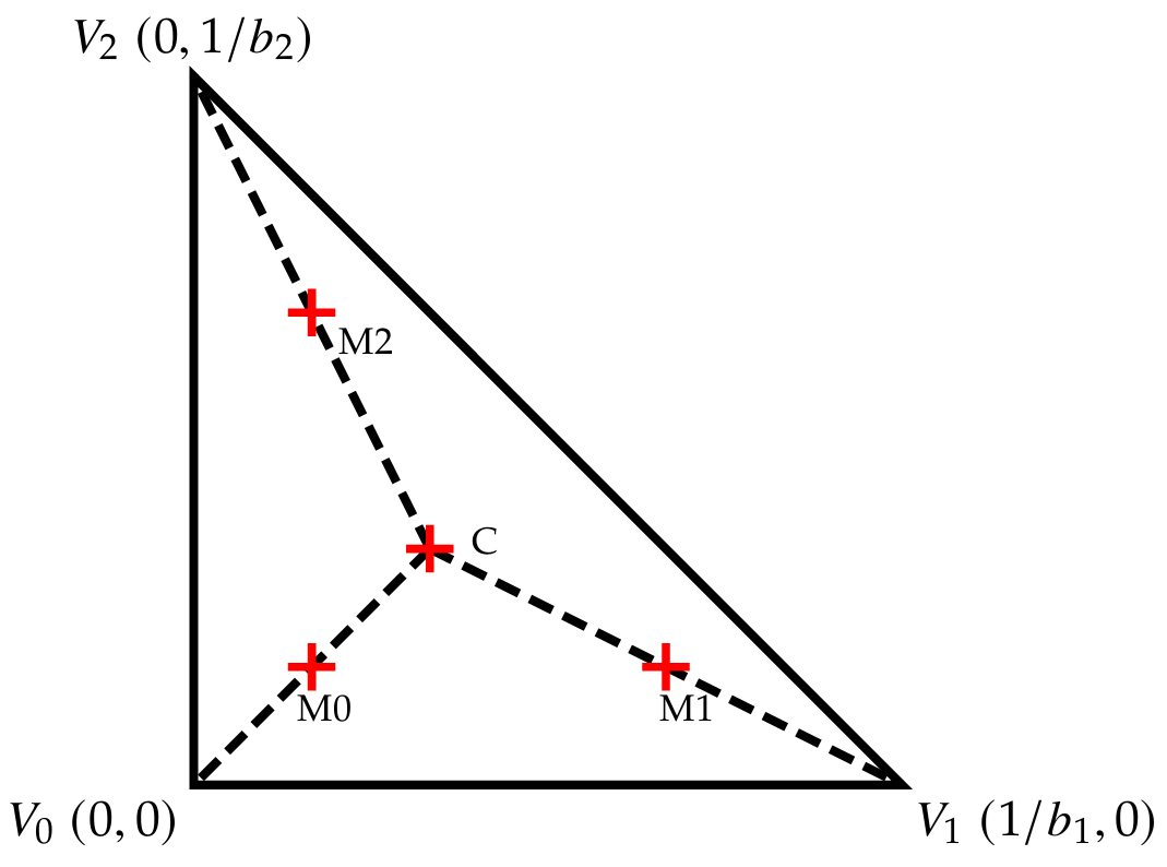
When instability is found, the trial-phase concentrations and internal-energy density are valuable information. They describe what kind of phase wants to appear. To turn that infinitesimal direction into a finite flash initial guess, the method assigns a trial volume, converts densities to extensive energy and mole amounts, subtracts them from the totals to obtain the bulk phase, and reduces the trial volume until the two-phase initial state has higher entropy than the single-phase state.
Reformulating entropy maximization in TVN variables
For clarity, consider phases at a common temperature . Volume and mole conservation can be built directly into the last phase:
The remaining internal-energy constraint is
with optimization variables
The constrained problem becomes
where is the sum of phase entropies after volume and mole balances have been eliminated. Introduce
At first sight this appears to add a new unknown, . The temperature stationarity equation removes it.
The Lagrange multiplier is
Stationarity with respect to temperature gives
Using the Helmholtz thermodynamic identities, both derivatives contain the sum of phase heat capacities at constant volume, and the ratio simplifies exactly to
This result is more than an algebraic convenience. It removes from the unknown vector and connects the energy constraint to the reciprocal temperature, the intensive variable thermodynamically conjugate to internal energy.
Substituting yields
With , the expression reduces to
—the Helmholtz-energy Q-function associated with the constrained problem. The published formulation denotes it . It has the form introduced by Michelsen, but here it emerges directly from one Lagrange multiplier in TVN space.
The entropy form and Helmholtz form are mathematically equivalent. The Helmholtz form is cheaper to evaluate because it needs for each phase rather than separate evaluations of and .
Why a saddle point is the correct target
After the constraints are embedded, equilibrium is found by solving
The solution is generally a saddle point, not an unconstrained maximum in every coordinate. This is expected: the original entropy is maximized only along the feasible manifold defined by fixed total energy. A Newton method solves the stationarity equations using the Hessian of the Q-function, often with line search or trust-region safeguards.
A useful consistency check is obtained by differentiating the reduced function:
- temperature stationarity recovers , the total-energy constraint;
- volume stationarity gives ;
- mole-number stationarity gives ;
- the use of one common already imposes thermal equilibrium.
Thus the reformulation does not approximate the thermodynamic conditions. It represents the same equilibrium in variables that match the EOS.
Newton’s method and practical safeguards
The nonlinear stationarity equations can be written as and solved by
Automatic differentiation can compute gradients and Hessians without finite-difference truncation. A backtracking line search selects to improve robustness. Several details remain important:
- phase volumes and mole numbers must remain admissible;
- a merit-function minimum is not automatically a physical equilibrium, so residual and thermodynamic checks are essential;
- tiny phases may need a controlled merge rule;
- stability must be rechecked after a phase split;
- for dynamic simulations, the previous time step is normally the best warm start.
The good initial phase split obtained from stability analysis was a major reason Newton’s method converged reliably in the test set.
Validation against published problems
The formulation was tested on six multicomponent problems and a pure-CO₂ case from the literature using a Peng–Robinson Helmholtz-energy implementation. The stability stationary points agreed closely with published reference data; the largest reported concentration discrepancy in the multicomponent stability cases was below .
The flash results reproduced phase temperatures, pressures, component distributions, volumes, energies, and entropies from the reference calculations. Equality of phase temperature and pressure emerged to the requested nonlinear tolerance, while the two-phase entropy was no lower than that of the unstable single-phase state.
This combination matters more than matching one scalar. A phase split is credible only when conservation, equilibrium, stability, and entropy direction all agree.
Where the speedup comes from
The TVN and conventional UVN formulations used comparable outer Newton iteration counts. Their cost differed because the UVN implementation repeatedly inverted inside derivative evaluations.
Across the reported cases, the conventional formulation required tens to more than one hundred inner temperature iterations; the TVN formulation required none. Representative line-search timings reported in the publication are:
| Problem | TVN Q-function | Conventional UVN, unscaled | Approximate speedup |
|---|---|---|---|
| P1 | 0.18 ms | 2.20 ms | 12× |
| P4 | 0.14 ms | 1.83 ms | 13× |
| P5 | 1.23 ms | 40.19 ms | 33× |
| P6 | 0.68 ms | 15.93 ms | 23× |
| Pure CO₂ | 0.05 ms | 1.00 ms | 20× |
Absolute timings depend on implementation, derivatives, solver settings, and hardware. The structural result is more general: if temperature is an explicit outer variable, derivative evaluation does not need to solve an implicit temperature problem.
TVN variables are also naturally better scaled. Temperatures usually remain on the order of hundreds of kelvin, whereas internal energies can be large, negative, or positive depending on the reference convention. This does not eliminate all scaling concerns, but it avoids one particularly awkward variable.
What this formulation does—and does not—solve
The reformulation provides an efficient equilibrium calculation once an appropriate phase count and initial guess are available. It does not make phase stability trivial, guarantee convergence from arbitrary guesses, or remove the need for phase appearance and disappearance logic. Near critical points, small phase fractions, nearly singular Hessians, and flat thermodynamic directions can still challenge a nonlinear solver.
It also does not by itself create a pipeline model. The next step is to call the stability and flash routines repeatedly inside a finite-volume flow solver, choose variables suited to cellwise extensive data, calculate an equilibrium mixture sound speed, and verify the resulting wave structure. That coupling is the subject of the next article.
The broader lesson is that the best mathematical formulation is often found by aligning the optimization variables with the constitutive model. UVN remains the physical specification. TVN is the computational coordinate system. The reformulation preserves the former while exploiting the latter.