Research notes
From four equilibrium equations to one: faster pure-CO₂ depressurization
How the saturation curve reduces the pure-component UV flash, how differentiating the constraint yields a temperature ODE, and where the efficiency–conservation trade-off appears.
During a CO₂ pipeline depressurization, a finite-volume solver advances density, momentum, and total energy. It does not directly advance temperature or vapour fraction. These must be reconstructed from thermodynamics, often by solving a nonlinear equilibrium problem in every cell and at every time step.
For pure CO₂, that standard calculation can be simplified dramatically. The key geometric fact is that vapour–liquid equilibrium has only one thermodynamic degree of freedom: all equilibrium states lie on the saturation curve. This article explains how that fact reduces the full equilibrium problem to one scalar equation, and then goes one step further by turning the constraint into a temperature evolution equation.
The work was published as A new temperature evolution equation that enforces thermodynamic vapour–liquid equilibrium in multiphase flows – application to CO₂ modelling in Computers & Fluids. A local copy is available here.
Why the usual closure is expensive
For a pure fluid in two-phase equilibrium, suppose the flow solver provides mixture density and mixture specific internal energy . A direct formulation solves for four unknowns:
where is vapour volume fraction and , are the phase densities. The equations impose mixture mass and energy together with equality of phase pressure and Gibbs free energy:
This is a UV-type flash written in density variables. It is physically direct, but solving four coupled nonlinear equations thousands of times per step is expensive, particularly with a detailed Helmholtz-energy equation of state such as Span–Wagner.
The saturation curve removes three unknowns
Along the pure-component saturation curve, temperature determines the coexisting pressure, phase densities, and phase energies:
Pressure equality and Gibbs-energy equality are already encoded in these saturation relations. For a specified mixture density, the volume fraction follows explicitly from the lever rule:
Substituting this expression into the mixture-energy equation leaves only one unknown, . Define
Then the two-phase closure is the scalar equation
In a single phase, the same notation can be extended with . The closure therefore becomes
in both regimes, with a piecewise definition of . I call this the Reduced-VLE-Algebraic formulation. It replaces a four-unknown nonlinear system by a one-dimensional root solve.
From an algebraic constraint to a temperature equation
The scalar equation is already cheaper, but it still requires a nonlinear solve. The next idea starts from the fact that the flash is embedded in a time-dependent simulation. Density, energy, and temperature are functions of time, so differentiate the equilibrium identity:
Solving for the temperature derivative gives
This is the Reduced-VLE-ODE formulation. If the initial condition satisfies the equilibrium constraint and the differential equation is integrated exactly, the trajectory remains on the equilibrium manifold. Numerically, the method evolves temperature together with the flow variables and avoids a dedicated nonlinear flash solve.
Coupling the equation to a finite-volume pipe model
For a pipe cell, the conservative semi-discrete equations supply
where the are the finite-volume flux residuals. Since
the internal-energy rate can be assembled from the three conservative rates. The resulting cellwise temperature equation is
The important implementation detail is that the pressure used in the flux still comes from the same thermodynamic state. The method is not “fluid dynamics first, temperature correction later.” Temperature is part of the coupled ODE state and affects the flux at each stage.
For a tank, the same construction is even clearer. Mass and energy balances provide and from inlet/outlet flow and heat transfer. Substitution into the boxed equation closes the model without an algebraic flash solve.
Three formulations, three numerical properties
| Method | Two-phase thermodynamic unknowns | Main strength | Main cost or risk |
|---|---|---|---|
| Full-VLE-Algebraic | Direct, constraints solved to nonlinear tolerance | Four-variable nonlinear solve | |
| Reduced-VLE-Algebraic | Much cheaper while retaining algebraic enforcement | Depends on saturation correlations and still needs a scalar root solve | |
| Reduced-VLE-ODE | as an evolved variable | No flash root solve; integrates naturally with explicit time stepping | Constraint and energy drift from time-discretization error |
The reduced algebraic method remains conservative because total energy is advanced by the conservation law and temperature is reconstructed from that energy. In the ODE method, temperature is advanced directly. A finite time step introduces truncation error in the equilibrium manifold, and reconstructing internal energy from the updated state exposes that error as energy drift.
This distinction matters. Two methods can give nearly indistinguishable pressure profiles over a short simulation while having different long-time conservation properties.
Tank depressurization: seeing the thermodynamic path
In a tank blowdown, pressure and temperature initially fall through a single-phase region. When the saturation curve is reached, the trajectory follows it while vapour and liquid coexist. The process can then return to a single-phase gas as depressurization continues.
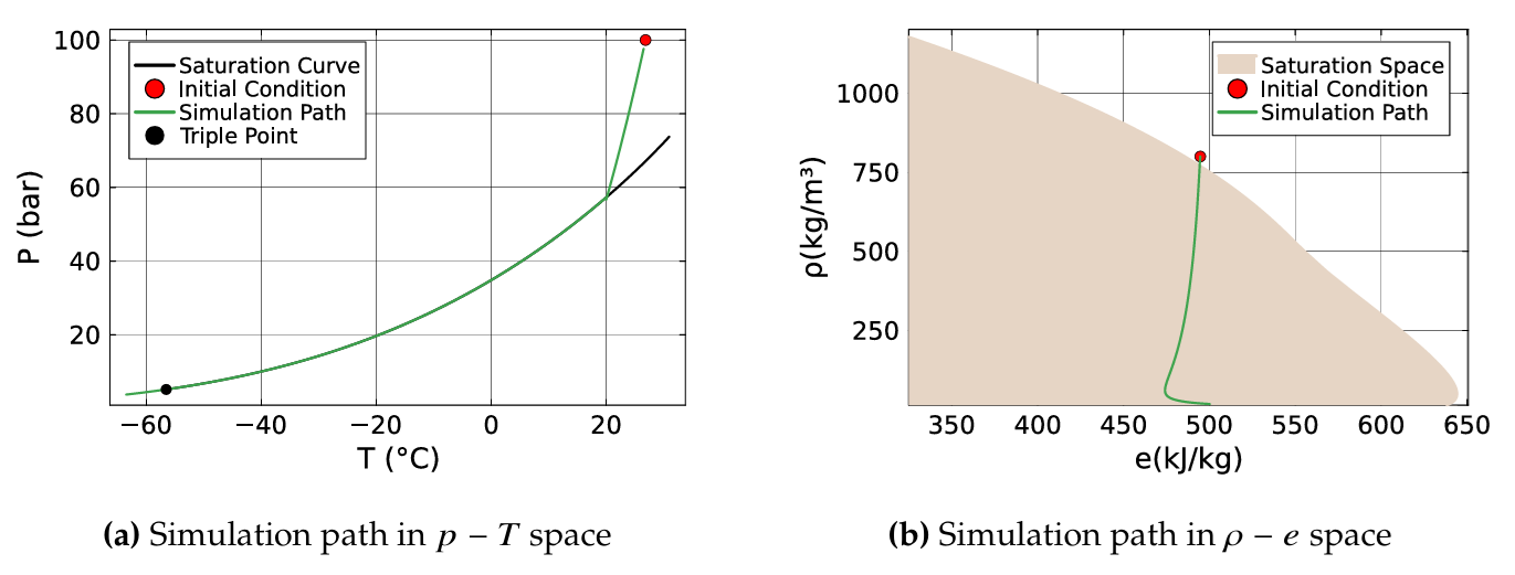
All three formulations reproduce the benchmark tank pressure and temperature histories closely. The reduced algebraic approximation inherits the small uncertainty of the saturation correlations. The ODE formulation adds time-integration error, especially when a trajectory crosses a phase boundary where thermodynamic derivatives change non-smoothly.
Accuracy versus computational cost
The reduced methods were approximately three to four times faster than the full four-variable flash in the studied cases. The algebraic and ODE reductions had comparable overall performance over much of the engineering-accuracy range.
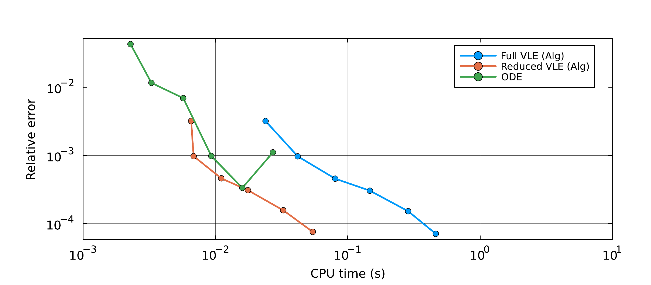
At tighter error targets, the ODE approach can lose some of its advantage because smaller time steps are needed near rapid phase transitions. This is a general lesson: removing a nonlinear solve does not remove stiffness or non-smooth thermodynamic behaviour; it changes where the computational difficulty appears.
What happens to energy conservation?
For a conservative finite-volume method in a closed shock tube, the algebraic formulations preserve the discretized total energy up to solver and round-off errors. The ODE method evolves temperature with a first-order time integrator. Its local temperature error is , which accumulates over steps into a global drift of approximately .
That does not make the ODE formulation unusable. It suggests a practical hybrid strategy:
- use the ODE update when the state evolves smoothly;
- monitor an energy or equilibrium residual;
- reduce the time step near a phase crossing;
- temporarily project back to the algebraic constraint if the residual exceeds a tolerance.
The algebraic formulation is the safer default when strict energy conservation is the priority. The ODE formulation is attractive when thermodynamic solves dominate cost and controlled drift is acceptable.
Phase change reshapes the Riemann solution
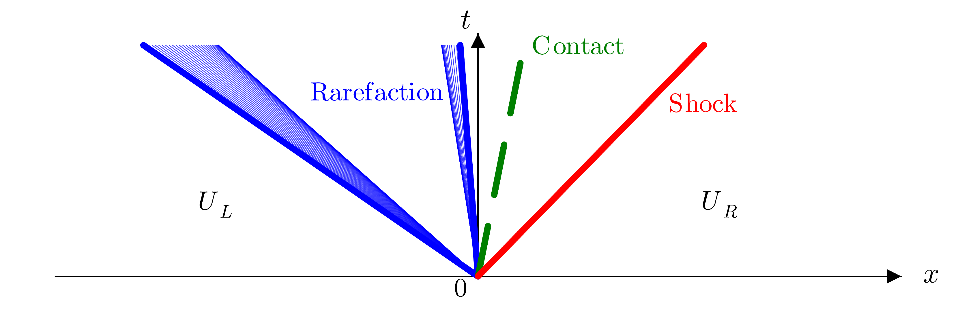
The pipeline shock-tube test contains a left-going rarefaction, a contact discontinuity, and a right-going shock. The rarefaction begins in single-phase liquid and crosses the saturation boundary. At that crossing, the equilibrium sound speed falls from roughly to in the reported case.
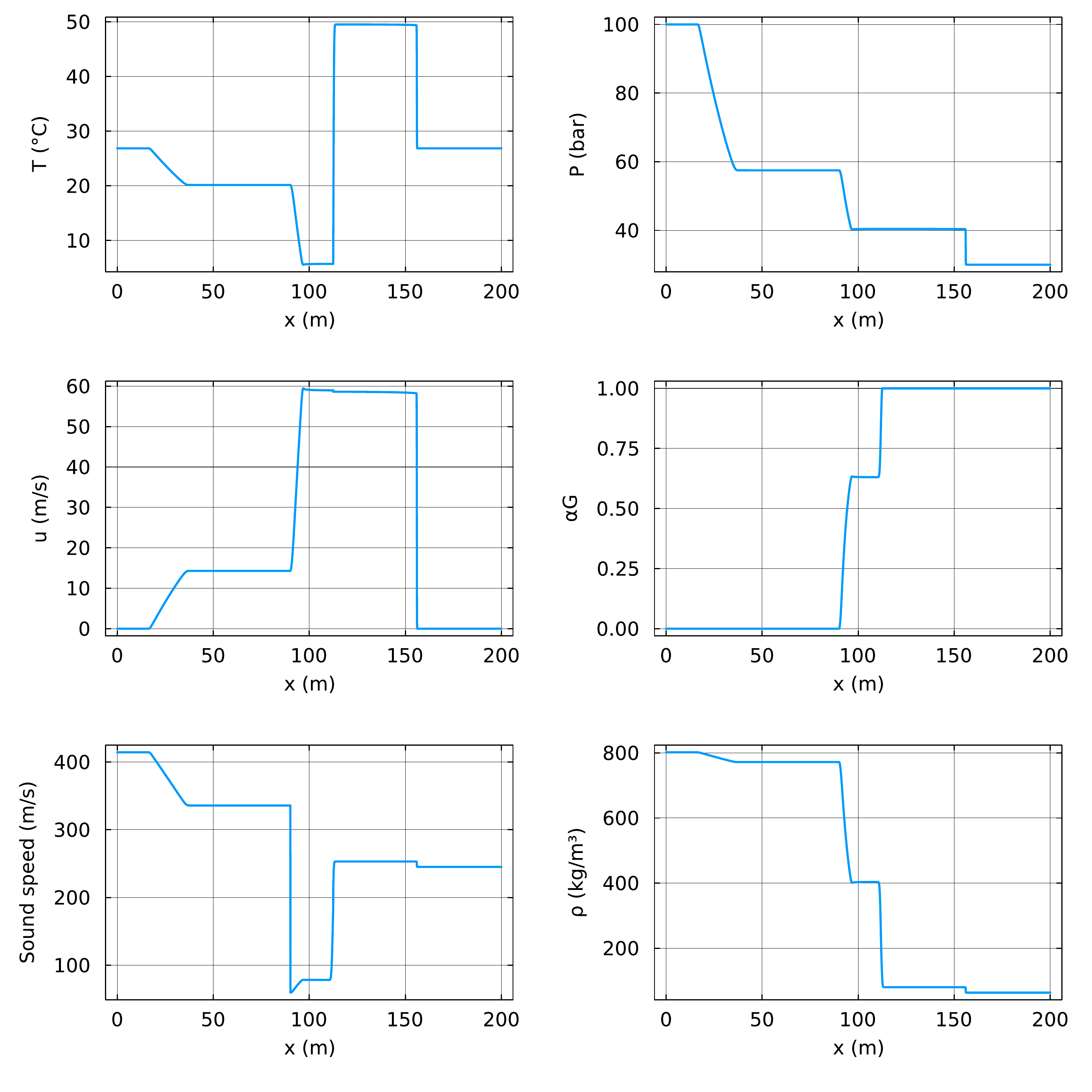
Because a finite interval of characteristic speeds is skipped by the sound-speed jump, the rarefaction separates into a single-phase fan and a two-phase fan with a constant intermediate state.
The same mechanism can be read in thermodynamic space. In the – plane the expansion reaches the saturation line and follows it. In the – plane the isentrope develops a kink at the phase boundary; since the isentropic slope determines sound speed, that kink explains the acoustic discontinuity.
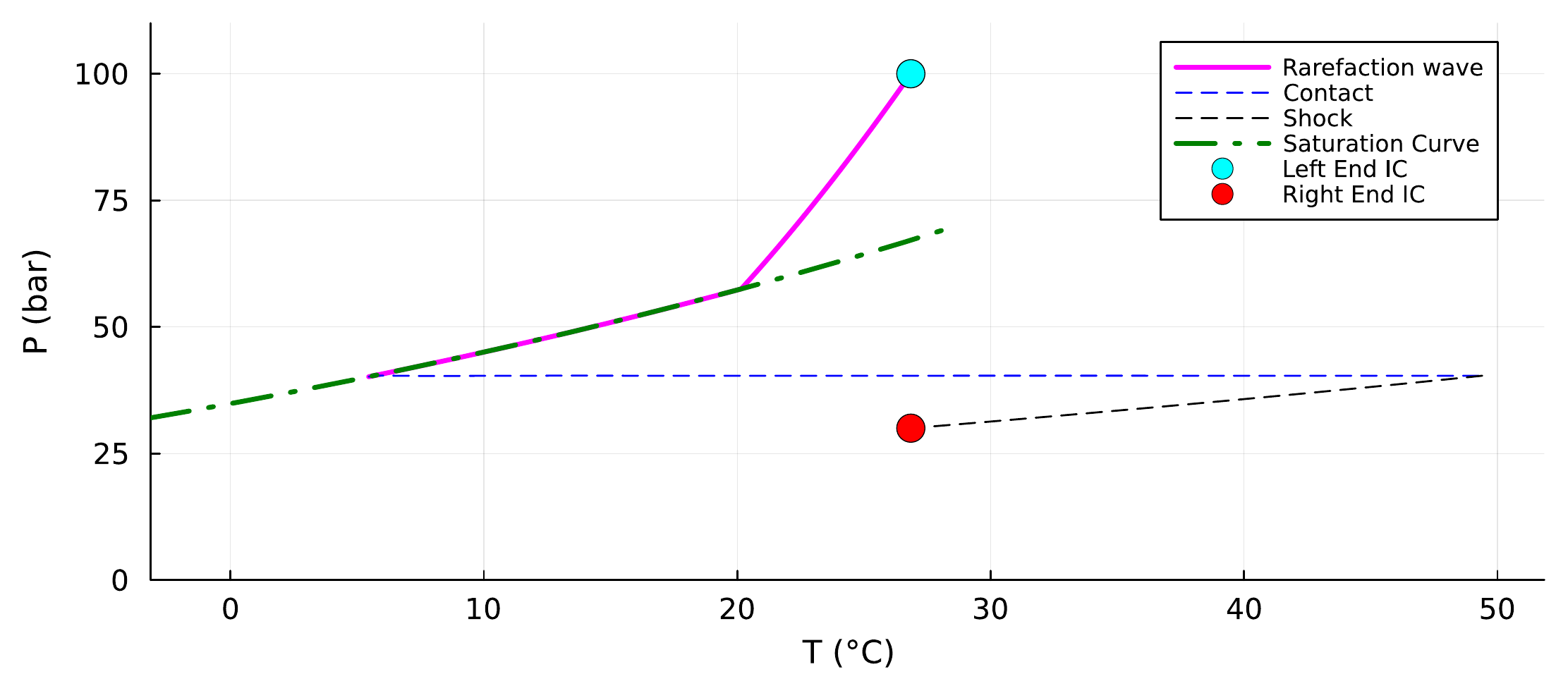
(a) Pressure–temperature profile
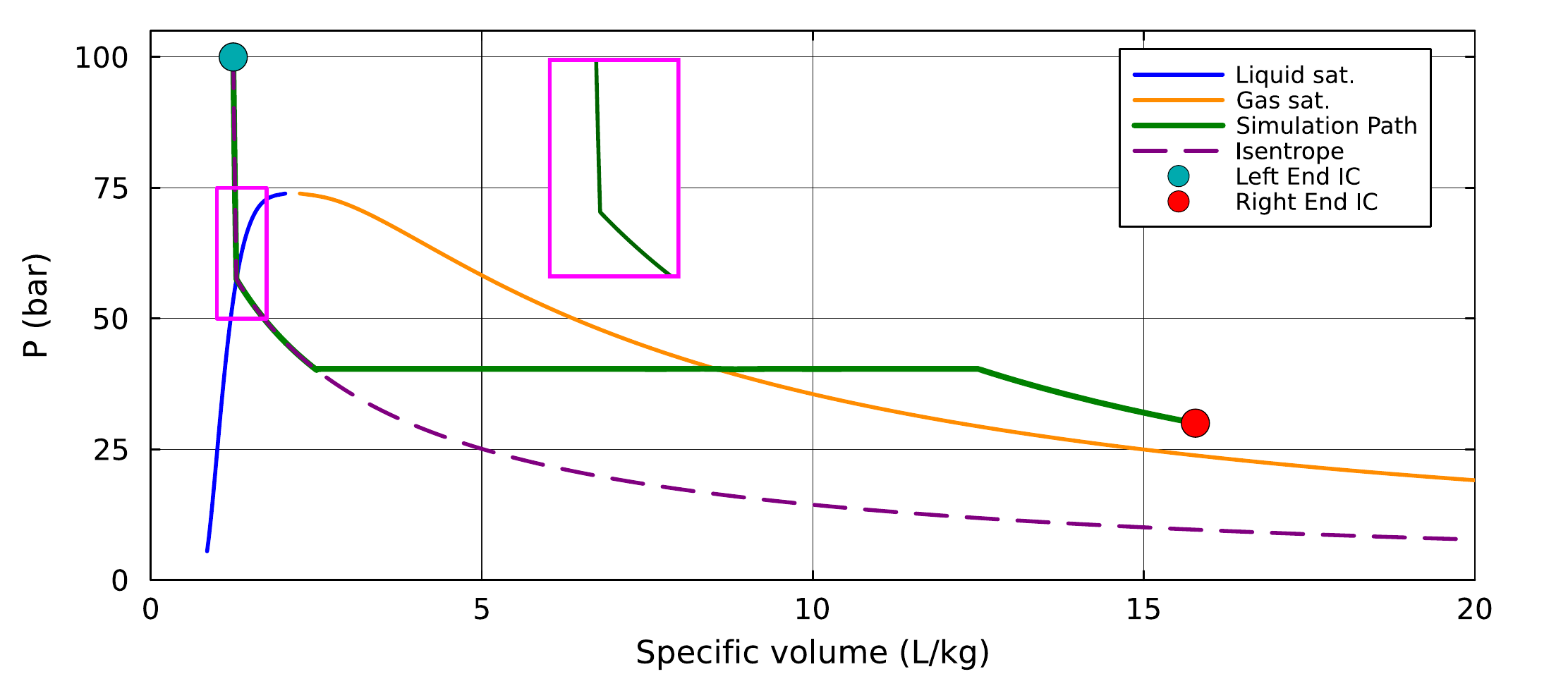
(b) Pressure–volume profile
Validation beyond idealized shock tubes
The reduced algebraic method was also compared with large-scale CO₂ release experiments from the Dalian facility. The cases cover gaseous and dense initial states, several orifice sizes, and full-bore rupture. A finite-orifice outlet condition permits choked two-phase discharge.
The simulations capture the main depressurization time scales and trends. Deviations are most visible in the fastest rupture cases and can partly reflect physical effects excluded from the model, especially heat transfer between the fluid, pipe wall, and surroundings. Validation therefore does more than award a pass or fail: it shows which missing physics becomes important in which regime.
Limits and the broader lesson
The reduction depends on accurate saturation relations and on the pure-component structure. It does not directly extend to CO₂-rich mixtures, where phase compositions vary independently. The ODE version also assumes enough regularity to differentiate the equilibrium relation, while phase boundaries introduce derivative discontinuities.
Nevertheless, the main idea generalizes: choose thermodynamic variables and constraints to match the geometry of the physical problem. For pure CO₂, the saturation curve turns a four-variable flash into one scalar relation. Differentiating that relation exposes an alternate dynamical formulation. The result is not merely a faster subroutine; it clarifies exactly where conservation, equilibrium, smoothness, and computational cost trade against one another.