Research notes
A unified model for two-phase transport of CO₂-rich mixtures
How HEM, a Helmholtz-energy EOS, stability analysis, a reformulated UVN flash, and equilibrium sound speed combine in multicomponent pipeline simulations.
The hardest part of a CO₂-rich pipeline simulation is not writing the conservation laws. It is closing them reliably when a depressurization moves thousands of cells through single-phase, near-critical, and vapour–liquid states while the composition of each equilibrium phase changes.
The published work brings the preceding developments into one framework:
- a finite-volume Homogeneous Equilibrium Model (HEM) for transient flow;
- a Helmholtz-energy Peng–Robinson equation of state;
- phase-stability analysis to decide whether a cell should split;
- a UVN flash reformulated in EOS-aligned variables;
- equilibrium and approximate mixture sound-speed calculations;
- tests on tanks, shock tubes, and published benchmark problems.
The associated article is A reformulation of UVN-flash for multicomponent two-phase systems with application to CO₂-rich mixture transport in pipelines. A local copy is available here.
One finite-volume update, two mathematical worlds
For an inviscid, adiabatic horizontal pipe, HEM evolves
with
A finite-volume cell update has the form
where the interface fluxes are computed here with an HLLC approximate Riemann solver.
The updated cell contains total mass, momentum, and energy. Thermodynamics needs temperature, phase volumes, and the amount of every component in each phase. The UVN flash translates from the conserved description to the equilibrium description. Pressure closes the flux; phase density and enthalpy support other model terms; and sound speed determines wave speeds and the stable time step.
The coupling is circular in a productive sense: fluxes update energy and density, the flash reconstructs pressure and phases, and those properties define the next fluxes.
The equation of state is phase-local
The Helmholtz free energy is written as
Its derivatives yield the properties needed by the flow and flash solvers:
An important implementation point is that an EOS describes a homogeneous phase. It cannot be evaluated once using two-phase mixture averages and expected to return equilibrium properties. If the cell is split, the EOS must be evaluated separately for gas and liquid using their own phase volumes and compositions. The flash calculation discovers those phase-local states.
Why the pure-CO₂ reduction no longer works for mixtures
For pure CO₂, a two-phase equilibrium state lies on a saturation curve. Temperature parameterizes saturation pressure and both phase densities. That geometry enabled a scalar reduced VLE equation.
For a mixture, vapour and liquid occupy a finite pressure–temperature envelope and have different compositions. A temperature does not uniquely determine the phase split. Every component adds a conservation constraint and a chemical-equilibrium condition. The multicomponent problem therefore needs the more general UVN framework described in the preceding article.
The cellwise flash workflow
After a flow update, each cell follows a guarded decision process.
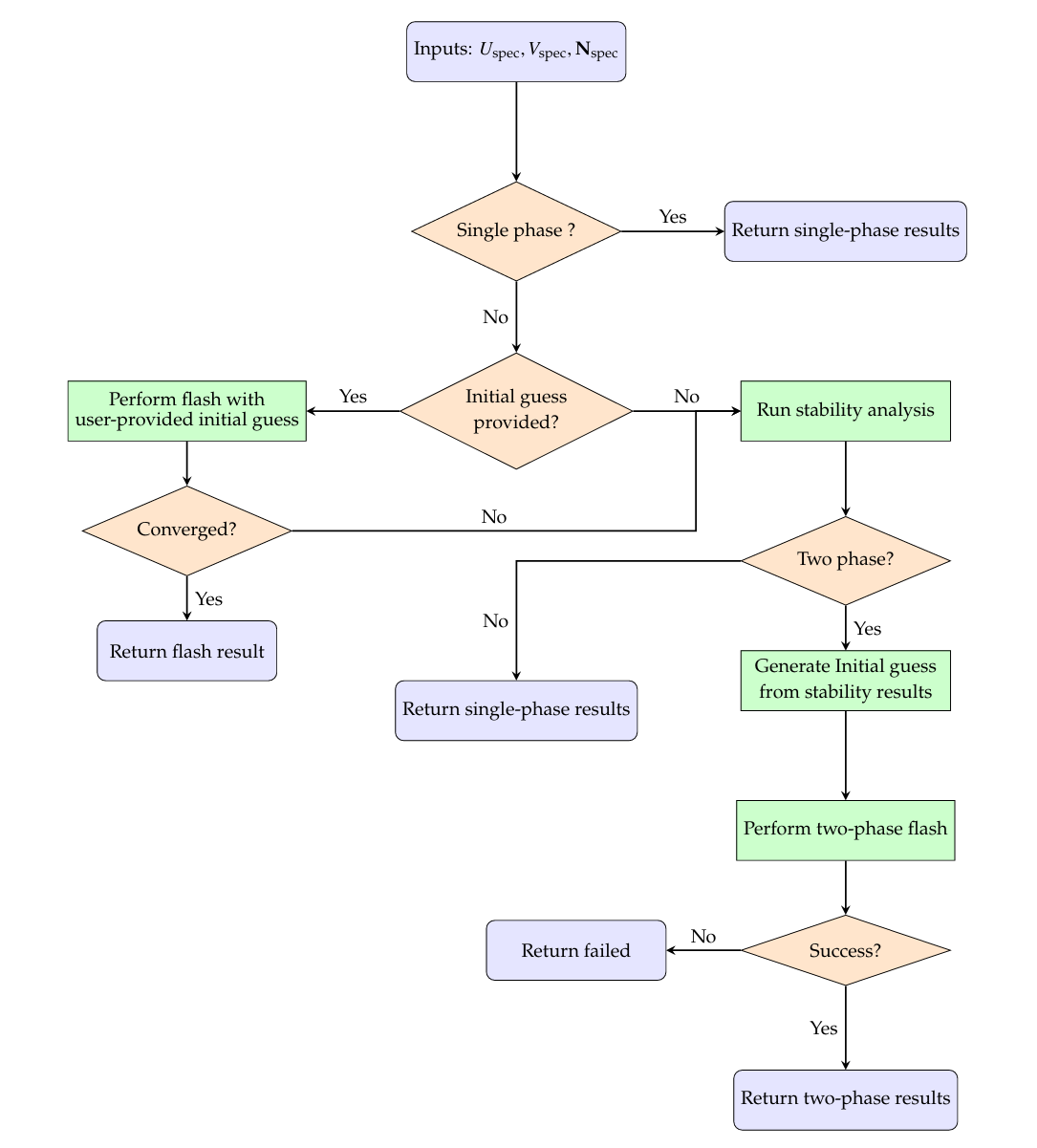
In words:
- Convert cell density, internal energy, volume, and overall composition into total , , and .
- If a reliable previous phase split is available, use it as a warm start.
- Otherwise evaluate the hypothetical single-phase state and run stability analysis.
- Return the single-phase properties if stable.
- If unstable, construct a two-phase initial guess from the stability stationary point.
- Solve the two-phase flash.
- Verify conservation and equality of intensive equilibrium quantities.
- If the nonlinear solve fails, return a controlled failure rather than silently accepting an unphysical state.
This logic is essential in a transient. Phase appearance is not a rare initialization event; a wave can cause neighbouring cells to enter or leave the phase envelope at successive time steps.
Pipeline-oriented flash variables
The general TVN reformulation uses common temperature, phase volumes, and phase mole numbers. For a pipeline cell, it is helpful to choose variables closer to the quantities used by the fluid solver and EOS implementation. The pipeline-oriented formulation uses
where is gas volume fraction and are gas-phase component molar densities. Liquid-phase component amounts follow from total component conservation:
and .
These variables have three practical advantages:
- has an immediate admissible range ;
- component densities are better scaled than raw extensive mole numbers when cell volume changes;
- gas and liquid EOS states can be assembled directly from phase volumes and compositions.
The flash still represents the same constrained entropy maximum. Stationarity recovers the specified total internal energy, equality of phase pressure, and equality of each component chemical potential.
Stable initialization across a moving phase boundary
The implementation combines three families of stability starts:
- simplex-based concentration guesses;
- saturation-pressure-based guesses;
- Gaussian perturbations of the single-phase concentrations.
Using diverse starts helps avoid the trivial stationary point and sample different incipient-phase directions. If instability is detected, the trial phase is assigned half the cell volume, then repeatedly reduced until the candidate split increases total entropy. In a time-dependent run, the converged split from the previous time step is usually even better.
Time integration and computational cost
The flow equations are integrated explicitly. At every stage, thermodynamic closure must be consistent with the stage state. The time step obeys a CFL restriction based on the largest local value of .
This leads to two distinct costs:
- number of flashes: proportional to cells × time steps × time-integration stages;
- cost per flash: stability starts, EOS derivative evaluations, and nonlinear iterations.
Warm starts reduce the second cost because most cells evolve only slightly during one stable time step. The difficult cells are concentrated near phase fronts, contacts, shocks, and near-critical states. This localization suggests later optimization strategies: cache single-phase decisions, reuse previous Hessian information, and devote more work only where the phase state can change.
Verifying the thermodynamic trajectory
Before comparing full spatial profiles, it is useful to examine the path of representative cells in pressure–temperature space. Literature shock-tube cases for CO₂–N₂ and CO₂–CH₄ mixtures cross different parts of their phase envelopes.
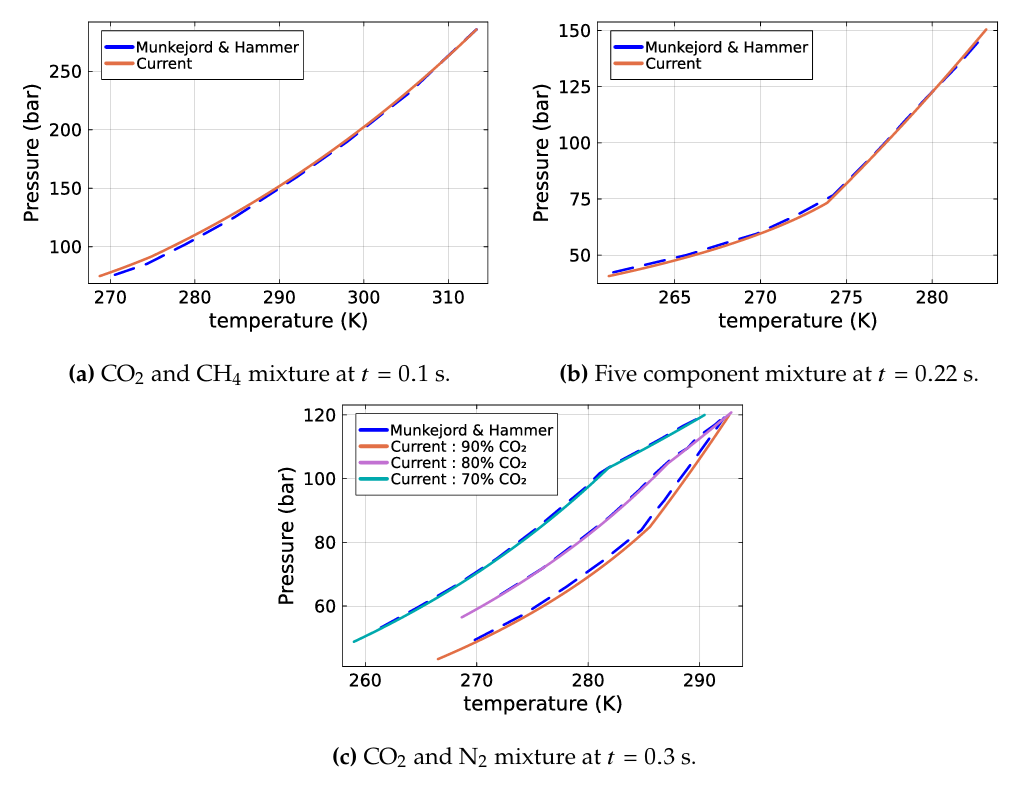
This plot is a valuable diagnostic. A phase fraction is meaningful only in relation to the phase envelope and conserved trajectory. If a profile reports two phases while its thermodynamic path remains outside the envelope, either the stability logic, plotting convention, or EOS evaluation needs investigation.
Sound speed: the thermodynamic derivative seen by the waves
In a single phase, isentropic sound speed is
For a two-phase equilibrium mixture, compression can change temperature, phase fraction, and phase compositions while maintaining entropy and total composition. The derivative must include all of those equilibrium responses.
Castier’s formulation writes
The derivative is obtained by differentiating the equilibrium conditions and solving a coupled linear system for the isentropic changes in temperature and phase composition. The same response can also be derived from the Jacobian of the converged flash equations. Their agreement is an independent consistency check linking the flash Hessian to the acoustic closure.
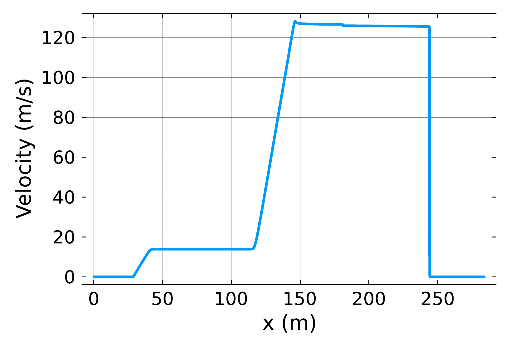
(a) Velocity profile
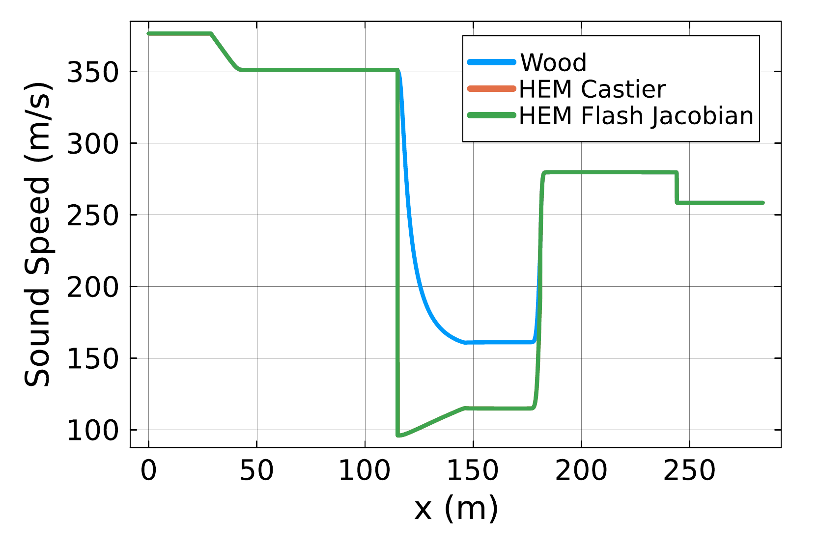
(b) Sound-speed profile
The classical Wood relation,
assumes mechanical equilibrium but does not fully represent thermal and chemical relaxation. It is much cheaper and, for the tested cases, produced very similar wave-speed estimates in the HLLC solver.
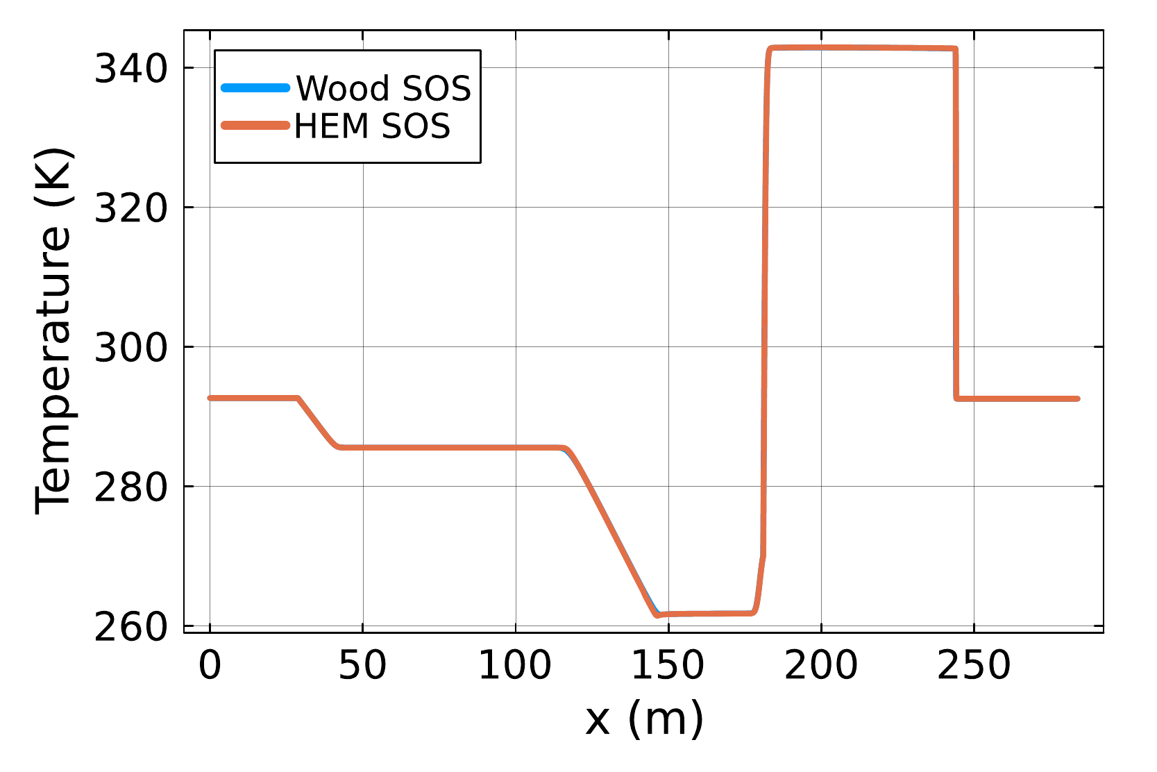
(a) Temperature profile
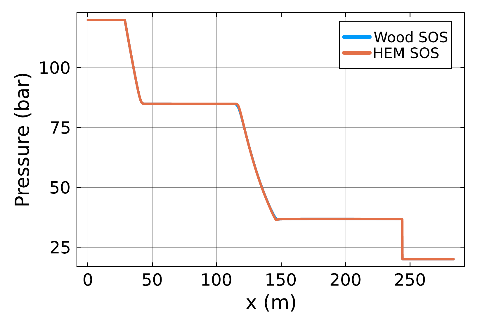
(b) Pressure profile
This agreement is useful but should not be universalized. Near critical conditions or for mixtures with stronger compositional response, the difference between frozen, mechanically equilibrated, and fully equilibrated acoustics may become important.
Reading the phase-transition region correctly
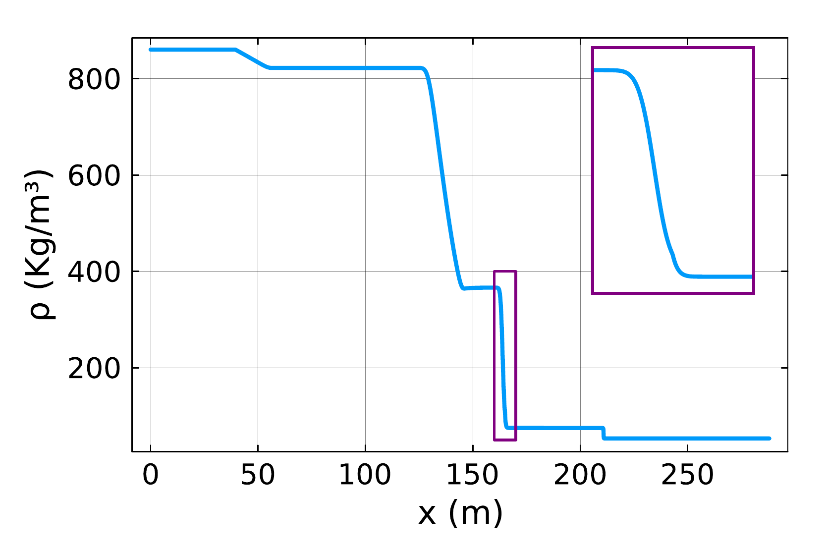
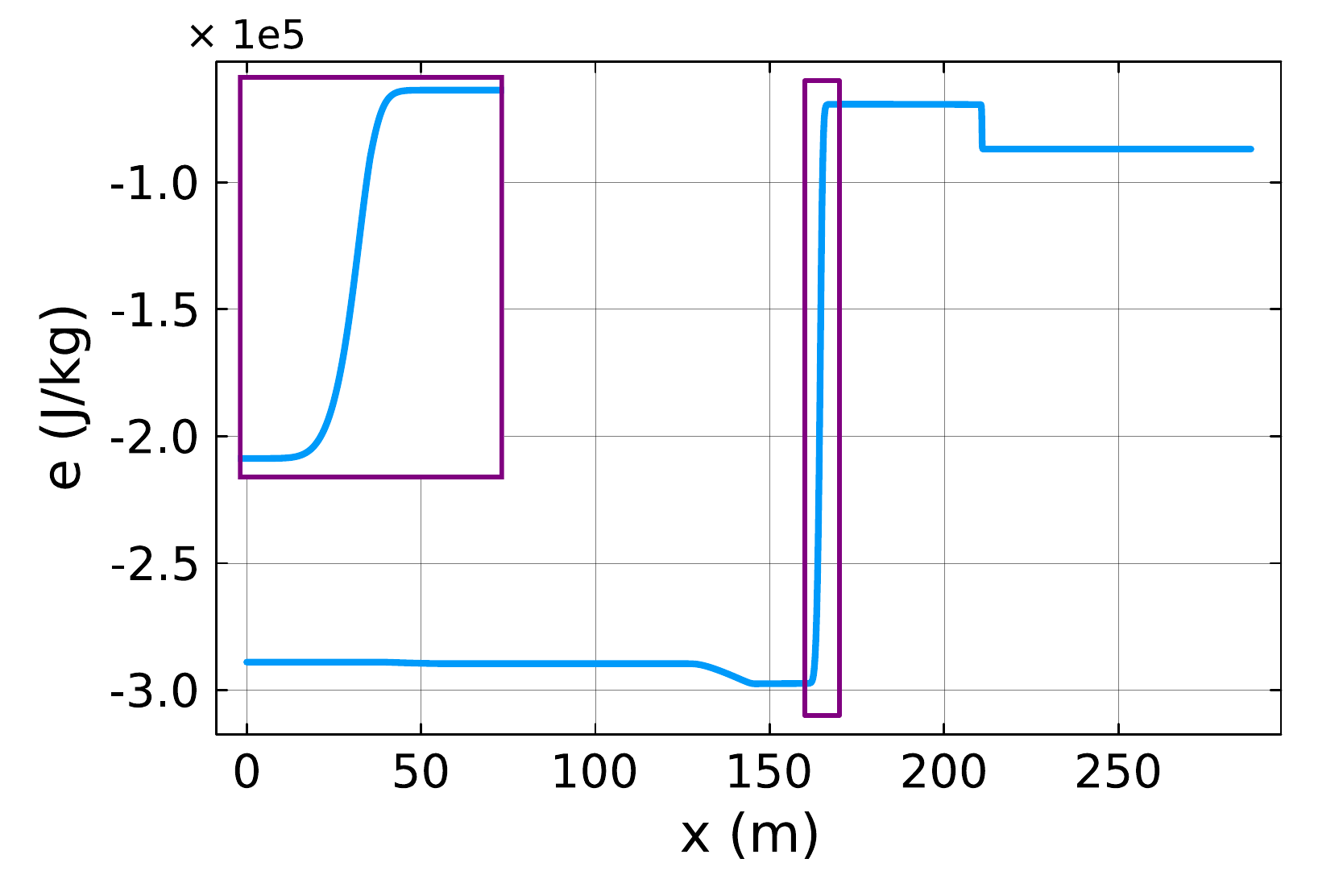
All shock-tube cases show the familiar large-scale pattern: a left-moving rarefaction, a contact discontinuity, and a right-moving shock. The subtle part is the narrow region between the rarefaction and contact, where liquid has expanded into a vapour–liquid mixture.
For pure CO₂, two-phase states lie on one saturation curve. At fixed saturation pressure and temperature, different vapour fractions can coexist depending on total energy and volume. Numerical smearing of a phase-fraction jump can therefore leave pressure and temperature almost unchanged.
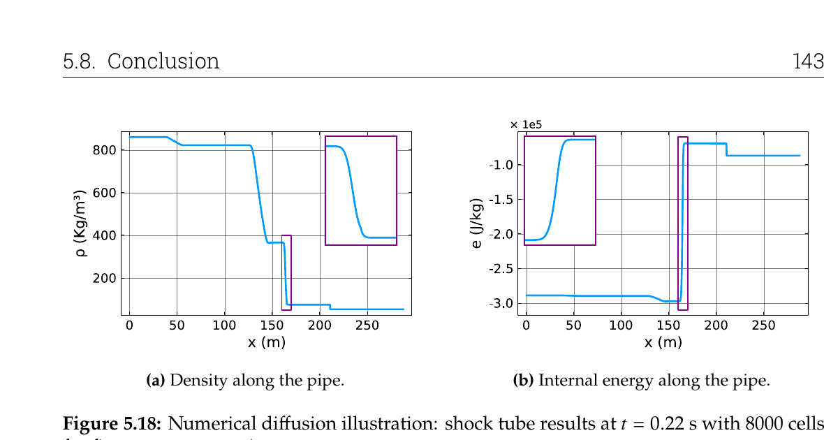
For a multicomponent mixture, two-phase states fill an envelope. At a fixed pressure and overall composition, changing equilibrium vapour fraction generally changes temperature. When a contact discontinuity is smeared across several finite-volume cells, the conserved density and internal energy vary smoothly across those cells. The UVN flash maps those intermediate conserved states to a sequence of equilibrium temperatures and phase fractions.
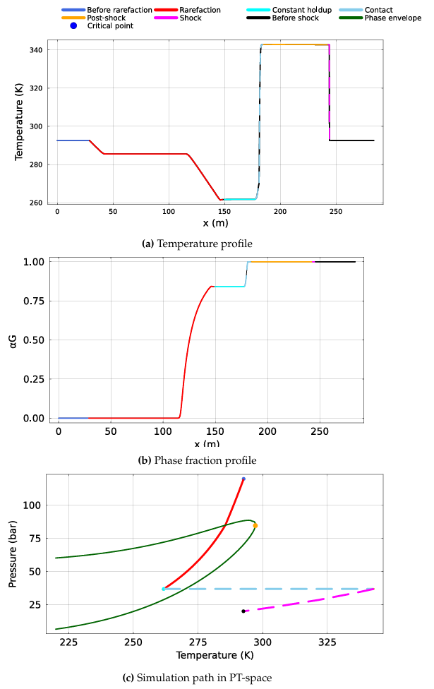
The resulting temperature slope can look like an additional physical wave. It is not. In the inviscid exact solution the contact contains a finite jump. The slope is the thermodynamic image of numerical diffusion in the conserved variables.
(a) Density profile
(b) Specific internal energy profile
This distinction is crucial when interpreting plots. A gradual phase-fraction curve is not automatically evidence of gradual physical evaporation. One must check mesh convergence, the width of the contact, and the corresponding path in thermodynamic space.
What the unified framework establishes
The numerical experiments support several conclusions:
- the reformulated UVN flash can serve as a practical closure inside a transient multicomponent flow solver;
- stability-derived and time-step warm starts make repeated phase splits robust;
- the HEM wave structure responds consistently to mixture composition and phase-envelope geometry;
- independent equilibrium sound-speed calculations agree, and Wood’s relation is an effective approximation for the tested HLLC cases;
- apparent smooth phase-transition zones must be separated into physical equilibrium response and numerical smearing.
Present limitations and next steps
The current model assumes instantaneous velocity, pressure, temperature, and chemical equilibrium between phases. It is one-dimensional and the highlighted shock-tube comparisons are inviscid and adiabatic. Real pipelines also involve wall friction, heat transfer, elevation, valves, junctions, potentially water or solid phases, and finite-rate relaxation. Peng–Robinson is efficient and broadly useful, but more accurate mixture models may be needed for detailed design across wider composition ranges.
Computationally, stability analysis and flash calculations remain the dominant cost. Future work can exploit temporal and spatial coherence: most cells stay in the same phase regime from one step to the next, and a phase front moves only locally. Parallelism, caching, adaptive stability checks, better scaling, and analytic or automatic derivatives can all help.
The main outcome is a consistent foundation. The flow solver and thermodynamic solver share the same conserved energy, composition, equilibrium assumptions, and sound-speed response. That consistency is what allows a pressure wave, a phase boundary, and a nonlinear flash calculation to be interpreted as parts of one physical solution rather than separate software modules.