Research notes

From Einstein’s equations to BSSN and FO-CCZ4

Why the covariant field equations are not yet a time-marching algorithm, and how ADM, BSSN, CCZ4, and FO-CCZ4 reorganize spacetime geometry into numerical evolution systems.

Published 18 July 2026

Einstein’s field equations fit on one line. A numerical-relativity code that solves them may contain tens of evolved fields, constraints, gauge equations, and thousands of derivative terms. The gap between those two descriptions is not a change in the underlying physics. It is a sequence of mathematical reformulations that turns a four-dimensional geometric statement into a well-posed initial-value problem on a three-dimensional grid.

This article follows that sequence:

\text{Einstein equations} \longrightarrow 3+1\ \text{split (ADM)} \longrightarrow \text{BSSN} \longrightarrow \text{CCZ4} \longrightarrow \text{FO-CCZ4}.

The aim is conceptual rather than benchmark-driven. No numerical results are presented yet. Instead, I describe what each variable represents, why it is introduced, and what numerical problem it helps to solve.

Gravity as spacetime geometry

In Newtonian physics, gravity is a force acting in an already existing space and time. In general relativity, gravity is encoded in the geometry of spacetime itself. Matter and energy influence that geometry, and freely falling objects follow the resulting geodesics.

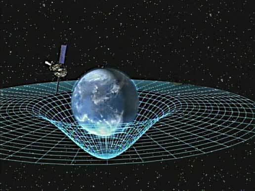
NASA illustration of Earth curving a grid used as an analogy for spacetime curvature — A common two-dimensional analogy for curved spacetime. It is useful for intuition, although real spacetime is four-dimensional and its curvature is not an embedding into an external space. Image credit: NASA, from What Is a Gravitational Wave?.

The central geometric object is the spacetime metric $g_{\mu\nu}$ . It tells us how to compute the invariant interval between nearby events:

ds^2=g_{\mu\nu}\,dx^\mu dx^\nu.

Throughout this article, Greek indices $\mu,\nu,\rho,\ldots$ run over spacetime coordinates $0,1,2,3$ , while Latin indices $i,j,k,\ldots$ run over spatial coordinates $1,2,3$ . Repeated upper and lower indices are summed. I use metric signature $(-,+,+,+)$ .

Einstein’s field equations

The field equations are

\boxed{ G_{\mu\nu}+\Lambda g_{\mu\nu} =\frac{8\pi G}{c^4}T_{\mu\nu} }

or, after expanding the Einstein tensor,

R_{\mu\nu}-\frac{1}{2}g_{\mu\nu}R +\Lambda g_{\mu\nu} =\frac{8\pi G}{c^4}T_{\mu\nu}.

Every symbol has a distinct role:

Symbol	Meaning	Intuition
$g_{\mu\nu}$	Spacetime metric	The local rule for measuring time, distance, angle, and causal structure
$g^{\mu\nu}$	Inverse metric	Raises indices and converts covectors into vectors
$R^\rho{}_{\sigma\mu\nu}$	Riemann curvature tensor	Measures how vectors change after parallel transport around an infinitesimal loop
$R_{\mu\nu}=R^\rho{}_{\mu\rho\nu}$	Ricci tensor	A contraction of curvature that records local volume focusing
$R=g^{\mu\nu}R_{\mu\nu}$	Ricci scalar	A scalar summary of Ricci curvature
$G_{\mu\nu}=R_{\mu\nu}-\tfrac12g_{\mu\nu}R$	Einstein tensor	The divergence-free curvature combination that matches local energy–momentum conservation
$T_{\mu\nu}$	Stress–energy tensor	Energy density, momentum density, stresses, and energy flux of matter and fields
$\Lambda$	Cosmological constant	A uniform spacetime-curvature contribution; often set to zero in local compact-object simulations
$G$	Newton’s gravitational constant	Sets the coupling strength between matter and geometry
$c$	Speed of light	Converts time and length units; numerical-relativity codes commonly set $G=c=1$

The slogan “matter tells spacetime how to curve; curved spacetime tells matter how to move” is useful, but the equations are mutually coupled. The matter fields evolve on $g_{\mu\nu}$ , while $T_{\mu\nu}$ sources the evolution of $g_{\mu\nu}$ .

Why the compact tensor equation is not yet a marching scheme

Writing $G_{\mu\nu}=8\pi T_{\mu\nu}$ does not identify which quantities should be supplied as initial data, which equations are constraints, which variables represent coordinate freedom, or how to compute a unique next time level. The equation is manifestly four-dimensional: space and time derivatives enter the same curvature tensor.

To see what the compact notation hides, start with the Christoffel symbols,

\Gamma^\rho{}_{\mu\nu} =\frac12 g^{\rho\sigma} \left( \partial_\mu g_{\sigma\nu} +\partial_\nu g_{\sigma\mu} -\partial_\sigma g_{\mu\nu} \right),

and the Ricci tensor,

R_{\mu\nu} =\partial_\rho\Gamma^\rho{}_{\mu\nu} -\partial_\nu\Gamma^\rho{}_{\mu\rho} +\Gamma^\rho{}_{\rho\lambda}\Gamma^\lambda{}_{\mu\nu} -\Gamma^\rho{}_{\nu\lambda}\Gamma^\lambda{}_{\mu\rho}.

Even the $00$ component expands to

\begin{aligned} R_{00}={}&\frac12\partial_\rho \left[g^{\rho\sigma} \left(2\partial_0g_{\sigma0}-\partial_\sigma g_{00}\right)\right]\\ &-\frac12\partial_0 \left[g^{\rho\sigma} \left(\partial_0g_{\sigma\rho} +\partial_\rho g_{\sigma0} -\partial_\sigma g_{0\rho}\right)\right]\\ &+\frac14 g^{\rho\sigma}g^{\lambda\kappa} \left(\partial_\rho g_{\sigma\lambda} +\partial_\lambda g_{\sigma\rho} -\partial_\sigma g_{\rho\lambda}\right) \left(2\partial_0g_{\kappa0}-\partial_\kappa g_{00}\right)\\ &-\frac14 g^{\rho\sigma}g^{\lambda\kappa} \left(\partial_0g_{\sigma\lambda} +\partial_\lambda g_{\sigma0} -\partial_\sigma g_{0\lambda}\right) \left(\partial_0g_{\kappa\rho} +\partial_\rho g_{\kappa0} -\partial_\kappa g_{0\rho}\right). \end{aligned}

Because $\rho,\sigma,\lambda,$ and $\kappa$ range over both $0$ and the spatial directions, this contains second time derivatives, second spatial derivatives, mixed derivatives such as $\partial_t\partial_i g_{\mu\nu}$ , and nonlinear products of first derivatives.

There is a second issue: coordinate freedom. Four functions’ worth of the ten metric components describe how coordinates are chosen, not independent physical gravitational degrees of freedom. Without gauge conditions, apparently different metric components can describe the same spacetime. The contracted Bianchi identities $\nabla_\mu G^{\mu\nu}=0$ also imply differential relations among the ten field equations.

ADM: slicing spacetime into space plus time

The Arnowitt–Deser–Misner (ADM) decomposition foliates spacetime by spatial hypersurfaces $\Sigma_t$ . Instead of trying to evolve a four-dimensional tensor all at once, we describe the geometry of one three-dimensional slice and how that slice sits inside spacetime.

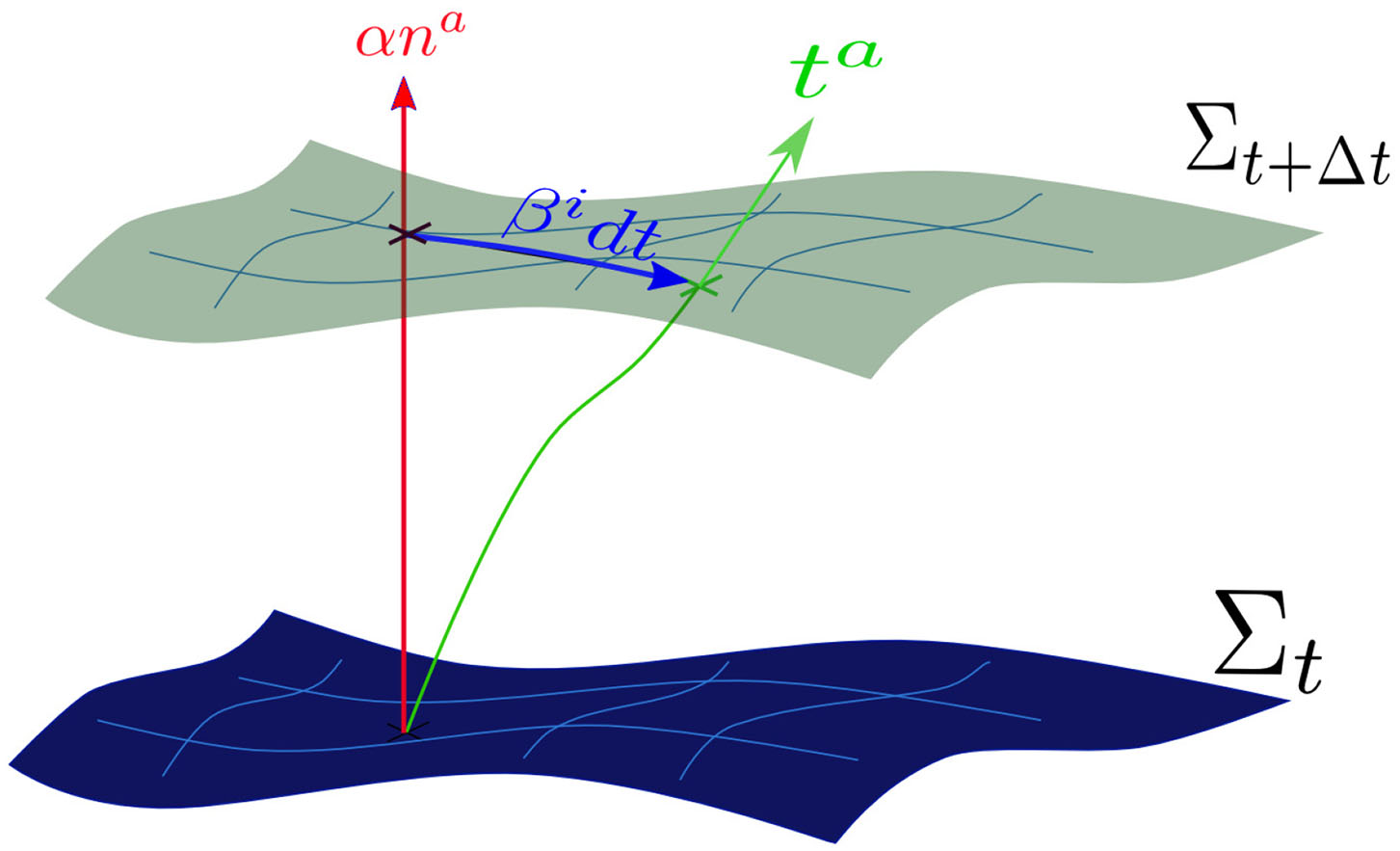
Two spatial hypersurfaces connected by lapse, shift, the normal vector, and the coordinate time vector — The 3+1 foliation. The lapse $\alpha$ advances proper time along the unit normal $n^a$; the shift $\beta^i$ moves spatial coordinates tangentially; the time vector is $t^a=\alpha n^a+\beta^a$. Figure from Carlos Palenzuela, Introduction to Numerical Relativity, CC BY 4.0.

The spacetime line element becomes

\boxed{ ds^2=-\alpha^2dt^2 +\gamma_{ij}(dx^i+\beta^i dt)(dx^j+\beta^jdt) }

with four basic ingredients:

$\gamma_{ij}$ is the spatial metric induced on $\Sigma_t$ . It tells us how rulers measure distance within one time slice.
$\alpha>0$ is the lapse. It specifies how much proper time elapses between neighbouring slices along their normal direction. Intuitively, it controls the rate at which coordinate clocks advance.
$\beta^i$ is the shift vector. It says how the spatial coordinate grid slides sideways from one slice to the next.
$n^\mu=(1/\alpha,-\beta^i/\alpha)$ is the future-directed unit normal to the slice.

The time-flow vector decomposes as

t^\mu=\alpha n^\mu+\beta^\mu.

Thus advancing one coordinate time step combines normal motion through spacetime with a tangential relabelling of spatial points.

Extrinsic curvature

The second dynamical ADM variable is the extrinsic curvature,

K_{ij} =-\frac12\mathcal L_n\gamma_{ij} =-\frac{1}{2\alpha} \left(\partial_t\gamma_{ij}-\mathcal L_\beta\gamma_{ij}\right).

$K_{ij}$ measures how the spatial geometry changes as the slices move through spacetime. A useful analogy is a two-dimensional surface: its intrinsic metric measures distances along the surface, while its extrinsic curvature describes how it bends within the surrounding geometry. In relativity the “surrounding geometry” is spacetime, and the sign depends on convention.

The trace

K=\gamma^{ij}K_{ij}

captures local volume expansion or contraction of the slice. The trace-free part captures directional shear.

ADM evolution equations and constraints

In geometrized units $G=c=1$ and with $\Lambda=0$ , the ADM evolution equations may be written

(\partial_t-\mathcal L_\beta)\gamma_{ij}=-2\alpha K_{ij},

\begin{aligned} (\partial_t-\mathcal L_\beta)K_{ij} ={}&-D_iD_j\alpha\\ &+\alpha\left({}^{(3)}R_{ij}+KK_{ij}-2K_{ik}K^k{}_j\right)\\ &-8\pi\alpha \left[S_{ij}-\frac12\gamma_{ij}(S-E)\right]. \end{aligned}

Here $D_i$ is the covariant derivative compatible with $\gamma_{ij}$ and ${}^{(3)}R_{ij}$ is its three-dimensional Ricci tensor. Matter is projected relative to $n^\mu$ :

E=n_\mu n_\nu T^{\mu\nu},\qquad S_i=-\gamma_{i\mu}n_\nu T^{\mu\nu},\qquad S_{ij}=\gamma_{i\mu}\gamma_{j\nu}T^{\mu\nu},

with $S=\gamma^{ij}S_{ij}$ . These are respectively the energy density, momentum density, and spatial stress seen by observers moving normal to the slice.

Four Einstein equations become constraints on every slice:

\boxed{ \mathcal H={}^{(3)}R+K^2-K_{ij}K^{ij}-16\pi E=0 }

and

\boxed{ \mathcal M_i=D_j(K^j{}_i-\delta^j{}_iK)-8\pi S_i=0. }

$\mathcal H$ is the Hamiltonian constraint and $\mathcal M_i$ are the three momentum constraints. Initial data must satisfy them. In free evolution, one advances the evolution equations and monitors the constraints rather than solving an elliptic system after every step.

ADM supplies the conceptual initial-value split, but its raw free-evolution form is not sufficiently robust for many long, three-dimensional simulations. Constraint-violating and gauge modes can grow. This motivates a better choice of variables.

BSSN: separating scale, shape, expansion, and shear

BSSN is named after Baumgarte, Shapiro, Shibata, and Nakamura. It starts from ADM but applies a conformal and trace-free decomposition designed to expose the structure that numerical evolution handles poorly in the raw variables.

Let

\gamma=\det(\gamma_{ij}),\qquad \varphi=\frac{1}{12}\ln\gamma.

Define the conformal spatial metric

\tilde\gamma_{ij}=e^{-4\varphi}\gamma_{ij}, \qquad \det(\tilde\gamma_{ij})=1.

This separates local scale from shape:

$e^{4\varphi}$ carries the local volume scale;
$\tilde\gamma_{ij}$ has unit determinant and carries anisotropic shape information.

Next split the extrinsic curvature:

K_{ij}=A_{ij}+\frac13\gamma_{ij}K,

and conformally rescale the trace-free part,

\tilde A_{ij}=e^{-4\varphi} \left(K_{ij}-\frac13\gamma_{ij}K\right), \qquad \tilde\gamma^{ij}\tilde A_{ij}=0.

Again the variables separate two effects:

$K$ is isotropic expansion or contraction;
$\tilde A_{ij}$ is trace-free distortion or shear.

Finally introduce the conformal connection functions

\tilde\Gamma^i =\tilde\gamma^{jk}\tilde\Gamma^i{}_{jk} =-\partial_j\tilde\gamma^{ij},

where the second equality uses $\det\tilde\gamma=1$ . Promoting $\tilde\Gamma^i$ to independent evolved variables is one of the decisive BSSN steps. It reorganizes troublesome Ricci-tensor terms and gives the gauge system direct access to coordinate distortions.

BSSN variable glossary

Variable	Components	Mathematical role	Physical or intuitive meaning
$\varphi$ (or alternatives $\chi=e^{-4\varphi}$ , $W=e^{-2\varphi}$ )	1	Conformal factor	Local spatial scale or volume element
$\tilde\gamma_{ij}$	6, with $\det\tilde\gamma=1$	Unit-determinant conformal metric	Shape of spatial geometry after scale is removed
$K$	1	Trace of extrinsic curvature	Local isotropic expansion/contraction of the slice
$\tilde A_{ij}$	6, with zero trace	Conformal trace-free extrinsic curvature	Direction-dependent shear of the evolving geometry
$\tilde\Gamma^i$	3	Contracted conformal connection	Spatial variation of conformal geometry; also drives coordinates
$\alpha$	1	Lapse gauge field	Rate of coordinate-time advance through the foliation
$\beta^i$	3	Shift gauge field	Sideways motion of coordinate labels across each slice

Before enforcing algebraic constraints, the usual BSSN state stores 17 conformal/geometric components plus gauge variables. Those stored components do not all represent independent physical degrees of freedom; the determinant, trace-free, connection, Hamiltonian, and momentum constraints restrict them.

What the BSSN evolution looks like

Some representative BSSN equations are

\partial_t\varphi =-\frac16\alpha K +\beta^k\partial_k\varphi +\frac16\partial_k\beta^k,

\partial_t\tilde\gamma_{ij} =-2\alpha\tilde A_{ij} +\beta^k\partial_k\tilde\gamma_{ij} +2\tilde\gamma_{k(i}\partial_{j)}\beta^k -\frac23\tilde\gamma_{ij}\partial_k\beta^k,

and, schematically,

\begin{aligned} \partial_t\tilde A_{ij} ={}&e^{-4\varphi} \left[-D_iD_j\alpha +\alpha({}^{(3)}R_{ij}-8\pi S_{ij})\right]^{\mathrm{TF}}\\ &+\alpha\left(K\tilde A_{ij} -2\tilde A_{ik}\tilde A^k{}_j\right) +\text{shift terms}, \end{aligned}

\partial_tK =-D^iD_i\alpha +\alpha\left(\tilde A_{ij}\tilde A^{ij}+\frac13K^2\right) +4\pi\alpha(E+S) +\beta^i\partial_iK.

The $\tilde\Gamma^i$ equation is longer. Its principal purpose is to turn derivatives of the conformal connection into their own evolution subsystem and to use the momentum constraint to replace certain derivatives of $\tilde A_{ij}$ . The resulting system has much better numerical behaviour with standard gauge choices than raw ADM.

Common moving-puncture gauges are

(\partial_t-\beta^i\partial_i)\alpha=-2\alpha K

for 1+log slicing, and a Gamma-driver system such as

\partial_t\beta^i=\frac34 B^i, \qquad \partial_t B^i=\partial_t\tilde\Gamma^i-\eta B^i.

The lapse prevents the coordinates from advancing too quickly into strongly curved regions, while the shift moves coordinate points to limit grid stretching. They are gauge conditions, not additional gravitational physics.

From BSSN to Z4 and CCZ4

BSSN monitors constraint violations but does not promote the four ADM constraints into a covariant dynamical field with explicit damping. The Z4 family introduces a spacetime four-vector $Z_\mu$ . The physical Einstein solution lies on the submanifold

Z_\mu=0.

In vacuum, a damped Z4 equation can be written schematically as

R_{\mu\nu} +\nabla_{(\mu}Z_{\nu)} +\kappa_1\left[ n_{(\mu}Z_{\nu)} -(1+\kappa_2)g_{\mu\nu}n_\rho Z^\rho \right]=0.

$\kappa_1$ sets a damping scale and $\kappa_2$ modifies the damping of different components. These terms vanish when $Z_\mu=0$ , so the continuum Einstein solution is unchanged. Away from the constraint surface, they are designed to propagate and reduce small resolved violations.

CCZ4 combines this Z4 mechanism with a BSSN-like conformal and trace-free split. Decompose

\Theta=-n_\mu Z^\mu, \qquad Z_i=\gamma_i{}^\mu Z_\mu.

$\Theta$ represents the normal, or energy-constraint-like, component of the Z4 field.
$Z_i$ represent its three spatial, or momentum-constraint-like, components.

Rather than evolve $Z_i$ separately, CCZ4 commonly folds it into

\hat\Gamma^i =\tilde\Gamma^i+2\tilde\gamma^{ij}Z_j.

If the constraints are satisfied, $\Theta=0$ , $Z_i=0$ , and $\hat\Gamma^i=\tilde\Gamma^i$ . A nonzero difference is therefore a dynamical measure of departure from the Einstein constraint surface.

Why make CCZ4 first order in space?

Standard BSSN and CCZ4 are first order in time but contain second spatial derivatives, for example in the spatial Ricci tensor and $D_iD_j\alpha$ . This is entirely compatible with finite differences and many production codes use it successfully.

High-order discontinuous Galerkin and finite-volume methods, however, are naturally formulated for first-order hyperbolic systems,

\partial_t\mathbf Q +A^1(\mathbf Q)\partial_1\mathbf Q +A^2(\mathbf Q)\partial_2\mathbf Q +A^3(\mathbf Q)\partial_3\mathbf Q =\mathbf S(\mathbf Q).

FO-CCZ4 introduces new variables for every required first spatial derivative. The price is a larger state vector; the reward is a system that is first order in both time and space and, with appropriate gauge and ordering-constraint choices, strongly hyperbolic.

The 58 FO-CCZ4 variables

The convention used in the original FO-CCZ4 formulation defines

\phi=(\det\gamma_{ij})^{-1/6}, \qquad \tilde\gamma_{ij}=\phi^2\gamma_{ij}.

This $\phi$ is related to the BSSN variable above by $\phi=e^{-2\varphi}$ . Keeping the two notations distinct avoids a common source of implementation errors.

The complete state vector is

\mathbf Q^T= \left( \tilde\gamma_{ij},\ln\alpha,\beta^i,\ln\phi, \tilde A_{ij},K,\Theta,\hat\Gamma^i,b^i, A_k,B^i{}_k,D_{kij},P_k \right).

Its variables can be understood in three groups.

1. Fields defining the four-metric: 11 variables

Variable	Count	Meaning
$\tilde\gamma_{ij}$	6	Unit-determinant conformal spatial metric; the shape of spatial geometry
$\ln\alpha$	1	Logarithmic lapse; evolving the logarithm guarantees $\alpha>0$ after exponentiation
$\beta^i$	3	Shift vector; coordinate-grid velocity within a slice
$\ln\phi$	1	Logarithmic conformal scale; guarantees $\phi>0$ and carries the spatial volume factor

In this FO-CCZ4 construction, these 11 quantities form a pure ODE subsystem: their equations contain algebraic functions of the full state but no spatial derivatives of these 11 fields themselves.

2. Curvature, constraint, and gauge-driver fields: 14 variables

Variable	Count	Meaning
$\tilde A_{ij}$	6	Trace-free conformal extrinsic curvature; anisotropic time deformation
$K$	1	Trace of extrinsic curvature; local volume expansion/contraction
$\Theta$	1	Normal component of Z4 constraint error
$\hat\Gamma^i$	3	Conformal connection augmented by the spatial Z4 field
$b^i$	3	Auxiliary Gamma-driver field controlling how the shift responds to connection distortion

$b^i$ is a coordinate-control variable, not a new physical field. Likewise, $\Theta$ and the $Z_i$ information inside $\hat\Gamma^i$ should vanish for an exact Einstein solution.

3. First-order derivative variables: 33 variables

A_i:=\partial_i\ln\alpha=\frac{\partial_i\alpha}{\alpha},

B^i{}_k:=\partial_k\beta^i,

D_{kij}:=\frac12\partial_k\tilde\gamma_{ij},

P_i:=\partial_i\ln\phi=\frac{\partial_i\phi}{\phi}.

Their counts and meanings are:

Variable	Count	Why that count?	Intuitive meaning
$A_i$	3	One spatial gradient	Spatial change of clock rate
$B^i{}_k$	9	A general $3\times3$ tensor; not symmetric	Spatial gradient of coordinate-grid velocity
$D_{kij}$	18	$k$ has 3 values and $ij$ is symmetric with 6 combinations	Spatial gradient of conformal geometry
$P_i$	3	One spatial gradient	Spatial change of conformal scale

The total is

11+14+33=58.

New variables create new constraints

Replacing derivatives by independent variables is exact only if the definitions remain satisfied:

\mathcal C^A_i=A_i-\partial_i\ln\alpha=0, \qquad \mathcal C^{B,i}{}_k=B^i{}_k-\partial_k\beta^i=0,

\mathcal C^D_{kij}=D_{kij}-\frac12\partial_k\tilde\gamma_{ij}=0, \qquad \mathcal C^P_i=P_i-\partial_i\ln\phi=0.

Because mixed partial derivatives commute for smooth fields, the auxiliary variables also satisfy curl or ordering constraints:

\partial_kA_i-\partial_iA_k=0,

\partial_kB^m{}_l-\partial_lB^m{}_k=0,

\partial_kD_{lij}-\partial_lD_{kij}=0, \qquad \partial_kP_i-\partial_iP_k=0.

In addition,

\det\tilde\gamma=1, \qquad \tilde\gamma^{ij}\tilde A_{ij}=0, \qquad \tilde\gamma^{ij}D_{kij}=0.

These are not bookkeeping details. Different combinations of the ordering constraints can be added to the evolution equations without changing the exact continuum solution. The original FO-CCZ4 derivation uses them carefully to obtain strong hyperbolicity. A naive “replace every derivative by a new symbol” reduction need not have the same mathematical quality.

Hyperbolicity and why it matters

For a first-order system, the principal symbol in a spatial direction $s_i$ is

A(s)=s_iA^i.

Strong hyperbolicity requires real characteristic speeds and a complete, uniformly well-conditioned set of eigenvectors. Informally, it means that the PDE has a controlled wave decomposition and a well-posed local initial-value problem. This is what allows errors and physical signals to propagate at identifiable characteristic speeds rather than growing arbitrarily at ever-smaller scales.

Strong hyperbolicity is a continuum property, not a guarantee that every discretization will be stable. Boundary conditions, gauge parameters, constraint damping, dissipation or limiters, resolution, and time integration still matter. Conversely, a high-order discretization cannot repair an ill-posed continuum formulation.

How the formulations relate

Formulation	Main variables	Spatial order	Central numerical idea
Covariant Einstein equations	$g_{\mu\nu}$	Second	Geometrically complete, but not yet an explicit gauge-fixed Cauchy algorithm
ADM	$\gamma_{ij},K_{ij}$ plus $\alpha,\beta^i$	Second	Separate spatial geometry, time evolution, and four constraints
BSSN	$\varphi,\tilde\gamma_{ij},K,\tilde A_{ij},\tilde\Gamma^i$	Second	Separate scale/shape and trace/shear; promote conformal connections
CCZ4	BSSN-like variables plus $\Theta$ and $Z_i$ information	Second	Propagate and damp violations of the Einstein constraints
FO-CCZ4	CCZ4 fields plus $A_i,B^i{}_k,D_{kij},P_i$	First	Strongly hyperbolic first-order system suited to DG and finite-volume methods

None of these formulations changes the physical solutions on the constraint surface. They change the off-constraint evolution, gauge dynamics, principal part, and numerical accessibility. Those differences determine whether inevitable truncation errors remain controlled during a long simulation.

A practical mental model

It is useful to attach one question to each layer:

Einstein: What spacetime geometries are compatible with the matter distribution?
ADM: What geometric data live on one spatial slice, and how do they evolve to the next?
BSSN: Which combinations of that data separate scale from shape and expansion from shear?
CCZ4: How should violations of the four Einstein constraints propagate and decay?
FO-CCZ4: Which gradient variables make every spatial derivative first order while preserving a strongly hyperbolic wave structure?

The apparent growth from one tensor equation to 58 evolution variables is therefore not unnecessary complication. Each layer exposes structure that the compact covariant notation deliberately hides.

What comes next

A later article can move from formulation to implementation: assembling the FO-CCZ4 state vector, generating initial data, enforcing algebraic and ordering constraints, selecting 1+log and Gamma-driver gauges, computing characteristic speeds, applying WENO or discontinuous Galerkin spatial discretization, choosing an SSP Runge–Kutta method, and monitoring Hamiltonian and momentum norms.

Before presenting results, the most important implementation audit is conceptual: every evolved variable should have one unambiguous definition, one consistent index symmetry, and one verified route back to the ADM metric and extrinsic curvature. That is the level at which many silent formulation-mixing errors begin.