Research notes

Why CO₂ pipeline transport is a thermodynamics problem

From CCS infrastructure and phase envelopes to Riemann waves, water hammer, and a proposed CO₂-hammer benchmark: an accessible map of the modelling problem.

Published 18 July 2026

Carbon capture and storage (CCS) is often summarized in three verbs: capture, transport, store. That description is correct, but it hides the part that makes transport scientifically interesting. A CO₂ pipeline is not simply a pipe carrying an ordinary liquid. Pressure waves, rapid cooling, impurities, and phase change can interact on the same time scale. A safe simulation must therefore solve a fluid-dynamics problem and a thermodynamic-equilibrium problem together.

This article introduces that coupled problem, using the water-hammer case and the corresponding CO₂-hammer benchmark as concrete illustrations of transient pipeline behaviour.

The transport link in the CCS chain

CCS is intended especially for emissions that are difficult to eliminate directly, including those from cement, steel, chemicals, and other energy-intensive industries. CO₂ is separated from an industrial stream, conditioned, moved to a storage site, and injected into a suitable geological formation. Transport connects geographically distributed emitters to storage capacity and therefore determines whether a regional CCS network can operate as one system.

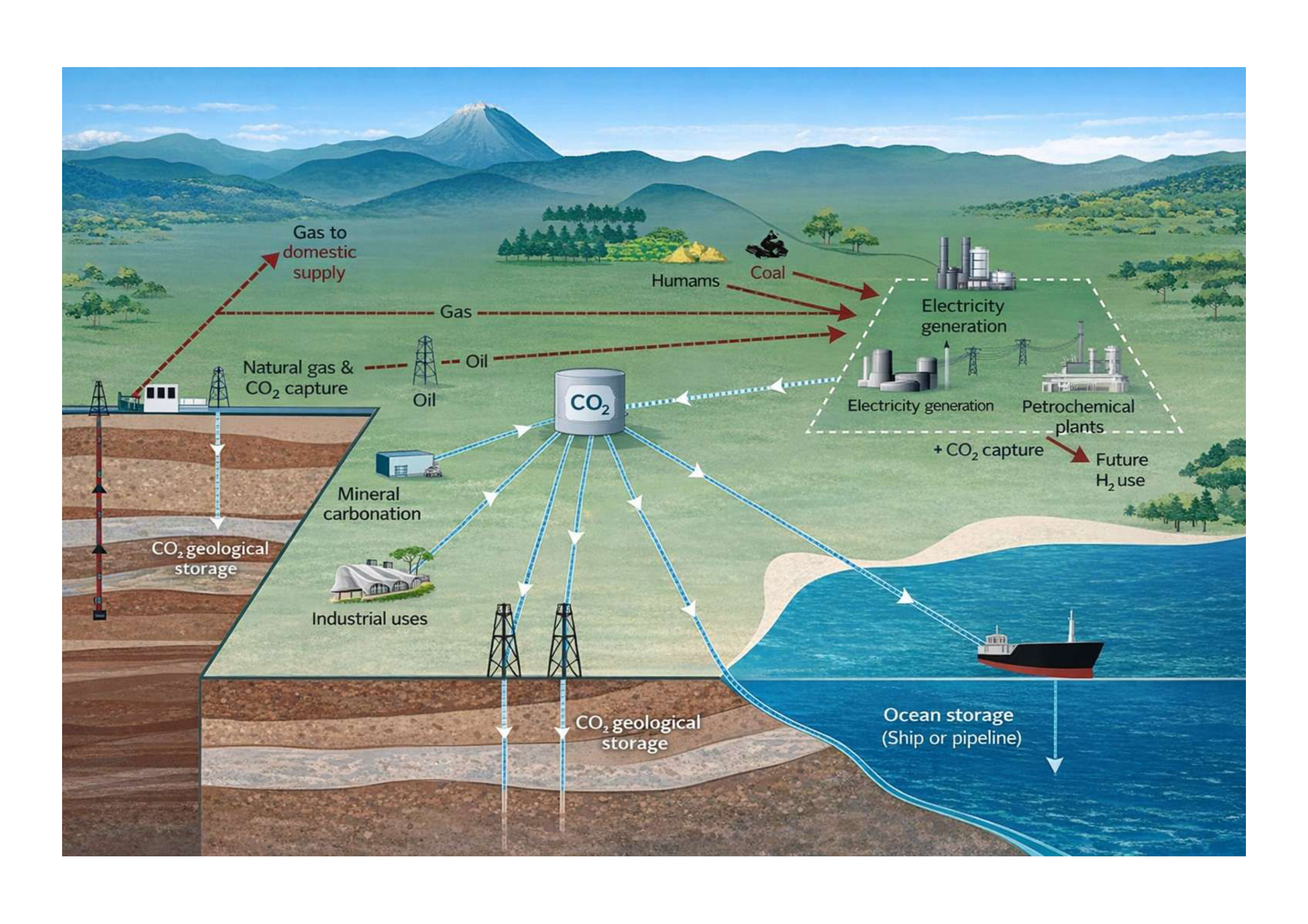
Illustration of carbon capture, pipeline and ship transport, and geological storage — The CCS chain from industrial sources to geological storage. Original illustration credited to the IPCC.

For small volumes or early projects, CO₂ can be moved by truck, rail, or ship. For sustained transport at the scale of millions of tonnes per year, pipelines are usually the natural choice. They are commonly designed to keep CO₂ dense, because high density increases transport capacity and reduces the volumetric flow rate. But “keep it dense” is an operating objective, not a guarantee. Start-up, shutdown, valve closure, accidental depressurization, terrain changes, heat transfer, or a rupture can drive the fluid through very different thermodynamic states.

That is where modelling becomes essential. Engineers need estimates of the highest pressure, the lowest temperature, the duration of a transient, the location and speed of a phase boundary, and the loads imposed on the pipe and connected equipment.

Captured CO₂ is a mixture

The phrase “CO₂ pipeline” can suggest a pure substance. Real captured streams contain impurities whose type and concentration depend on the source and capture technology. Possible components include nitrogen, oxygen, methane, water, hydrogen, carbon monoxide, hydrogen sulphide, argon, sulphur oxides, and nitrogen oxides.

Even a modest impurity level can change:

the critical pressure and temperature;
the width and location of the two-phase region;
mixture density and compressibility;
the speed of sound and therefore the propagation of pressure waves;
the temperatures reached during expansion;
corrosion, hydrate, and material-integrity risks.

For a pure component, vapour and liquid coexist on a saturation curve in pressure–temperature space. A multicomponent mixture instead has a finite phase envelope, bounded by bubble-point and dew-point curves. The envelope changes with composition.

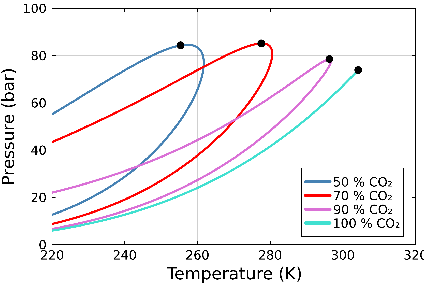
Pressure-temperature phase envelopes for carbon dioxide and methane mixtures — Peng–Robinson phase envelopes for CO₂–CH₄ mixtures. As the CO₂ mole fraction approaches 100%, the finite mixture envelope contracts toward the pure-CO₂ saturation curve.

This distinction is fundamental. For pure CO₂ in two-phase equilibrium, fixing temperature fixes saturation pressure. In a mixture, the same pressure can coexist with a range of equilibrium temperatures and phase fractions, depending on composition and the other conserved quantities. A thermodynamic routine that works for pure CO₂ cannot simply be relabelled as a mixture model.

Choosing a fluid model

A detailed two-fluid model can assign separate velocities, energies, and sometimes pressures to the gas and liquid phases. Such a model can represent slip, thermal disequilibrium, and finite-rate mass transfer, but it also introduces closure relations for interfacial drag, heat transfer, and relaxation. Those relations must be calibrated and validated.

At the other end of the hierarchy is the Homogeneous Equilibrium Model (HEM). In HEM, coexisting phases are assumed to share:

one velocity (kinematic equilibrium);
one pressure (mechanical equilibrium);
one temperature (thermal equilibrium);
equal component chemical potentials across phases (chemical equilibrium).

The mixture can then be evolved with Euler-type conservation laws for total mass, momentum, and energy:

\frac{\partial}{\partial t} \begin{bmatrix} \rho\\ \rho u\\ \rho E \end{bmatrix} + \frac{\partial}{\partial x} \begin{bmatrix} \rho u\\ \rho u^2+p\\ (\rho E+p)u \end{bmatrix} =0.

Here $\rho$ is mixture density, $u$ velocity, $E=e+u^2/2$ total specific energy, $e$ internal energy, and $p$ pressure. The equation looks compact, but it is not closed: after the conserved variables have been updated, the simulator still needs pressure, temperature, phase fractions, phase compositions, and sound speed.

HEM is attractive as a research and verification model because it isolates this coupling clearly. It is appropriate when relaxation to equilibrium is fast relative to the resolved flow. It is not a universal substitute for non-equilibrium models: strong phase slip or delayed evaporation may require a richer description. The useful question is not “Is HEM always true?” but “For which transients and length scales is its equilibrium assumption a defensible approximation?”

Why the flash calculation appears in every cell

Consider one finite-volume cell after a time step. The flow solver gives total volume, internal energy, and the amount of each component. In thermodynamic notation these are $U$ , $V$ , and $\mathbf N$ . The closure problem is therefore a UVN flash:

Given total internal energy $U$ , total volume $V$ , and component mole numbers $\mathbf N$ , determine the stable equilibrium state.

The calculation first asks whether a single phase is stable. If not, it determines how total energy, volume, and each component divide between the phases, subject to conservation and equilibrium. For two phases, the result must satisfy

T^{g}=T^{\ell},\qquad p^{g}=p^{\ell},\qquad \mu_i^{g}=\mu_i^{\ell}\quad \text{for every component }i.

This nonlinear calculation may be required in every cell at every time step. A pipeline simulation can therefore call the thermodynamic solver millions of times. Robust initialization and carefully chosen variables matter as much as the formal equilibrium equations.

Pressure disturbances are wave problems

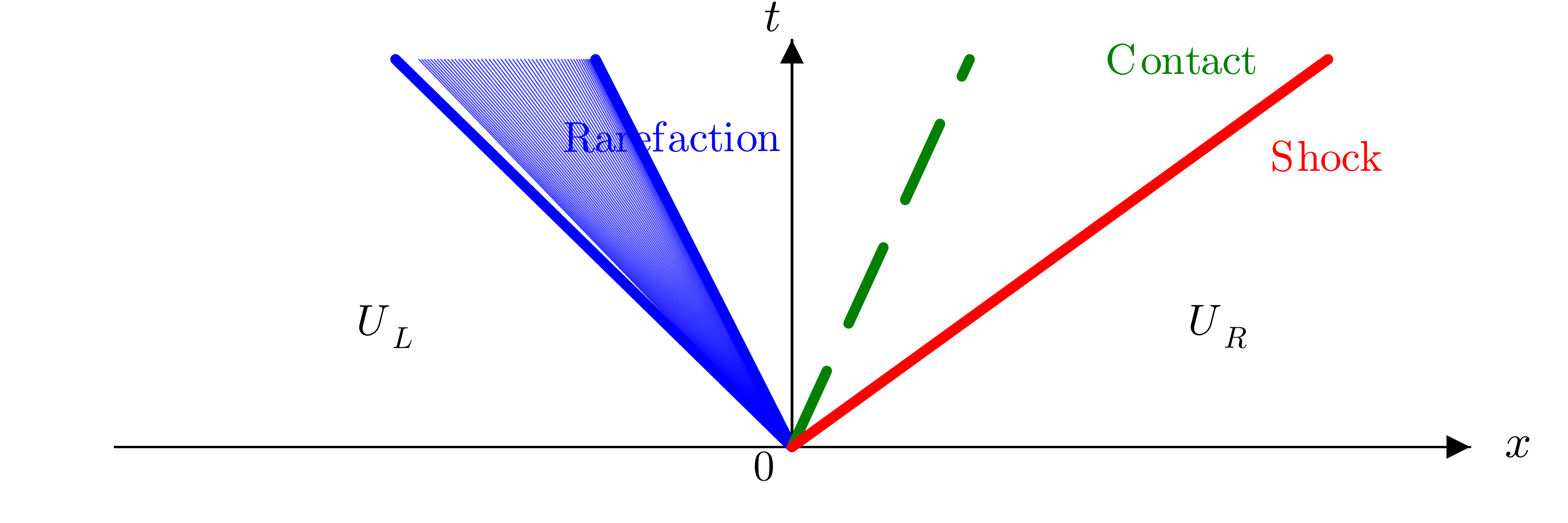
A sudden change at a valve or boundary does not affect the whole pipe instantaneously. Information propagates as waves. The idealized local problem is a Riemann problem: two constant states are separated by a discontinuity, and the solution is organized by characteristic waves.

For a classical single-phase Euler system, the three characteristic speeds are

u-c,\qquad u,\qquad u+c,

where $c$ is the speed of sound. These correspond to a left-running acoustic wave, a contact wave, and a right-running acoustic wave. Depending on the states, an acoustic wave can be a smooth rarefaction or a shock.

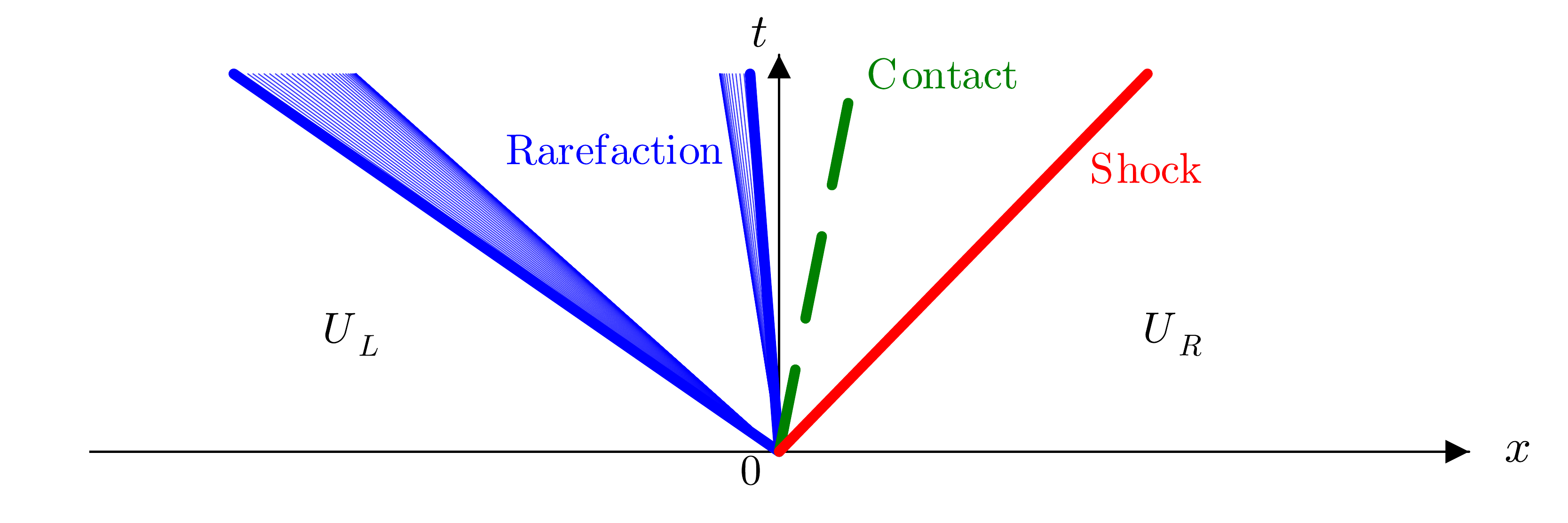
Single-phase Riemann wave structures — A classical Riemann solution for a single-phase system.

Two-phase Riemann wave structures — A classical Riemann solution for a two-phase system. When a rarefaction crosses a phase boundary, the sound-speed jump can split it into a composite structure.

Phase change complicates this picture because the equilibrium sound speed can change abruptly at a phase boundary. In a two-phase region the mixture is often much more compressible, so $c$ can fall sharply. A rarefaction crossing from liquid into a vapour–liquid state can therefore separate into two fans with a constant state between them. This is a composite rarefaction. It is not an extra conservation law; it is the wave-level signature of a non-smooth thermodynamic closure.

This is why sound speed is not merely a post-processing quantity. It enters the eigenvalues, numerical flux, CFL time-step restriction, wave positions, and boundary treatment.

Water hammer: the familiar reference case

Water hammer provides an intuitive transient benchmark. Imagine a pipe initially carrying liquid at steady velocity. Closing the outlet valve converts kinetic energy into compression. A pressure wave travels upstream, reflects from boundaries, and produces an oscillatory pressure history.

For an idealized rapid closure, the Joukowsky relation estimates the initial pressure rise:

\Delta p = \rho c\,\Delta u.

The relation is simple, but it exposes the key variables: density, sound speed, and velocity change. A numerical model should reproduce the pressure amplitude, travel time, reflections, and damping behaviour at the chosen level of physical modelling.

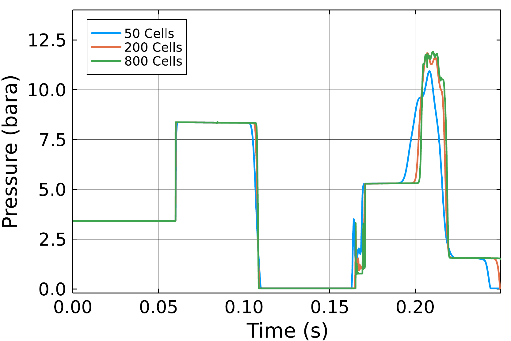
Mesh-refinement pressure histories for the Simpson water-hammer benchmark — Pressure just upstream of the outlet valve in Simpson’s water-hammer configuration. Results for 50, 200, and 800 cells show the mesh-convergence behaviour of the present model.

The benchmark is valuable precisely because the dominant physics is well understood. If the discretization, boundary condition, or wave speed is wrong, the error becomes visible in the timing and magnitude of the peaks.

From water hammer to CO₂ hammer

Now replace water by dense CO₂ and retain the sudden valve closure. Compression still launches a wave, but the low-pressure part of a reflection can intersect the saturation condition. Vapour forms; when pressure rises again, it condenses. The transient can therefore move repeatedly between dense single-phase and two-phase states.

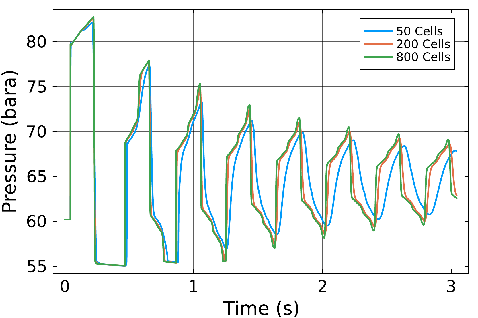
Mesh-refinement pressure histories for a proposed carbon-dioxide hammer test — The proposed CO₂-hammer counterpart to Simpson’s water-hammer case. The oscillation interacts with the saturation pressure, so the model repeatedly exercises phase appearance and disappearance.

This makes the CO₂-hammer case a demanding integration test. In one compact setup it tests:

the finite-volume wave propagation;
the inlet and closed-valve boundary conditions;
real-fluid properties and sound speed;
detection of phase instability;
robust switching between one- and two-phase calculations;
consistency between the conserved energy and the reconstructed thermodynamic state.

The water- and CO₂-hammer calculations show mesh convergence in the present model. The CO₂ case is especially informative because the fluid repeatedly crosses a phase boundary, directly testing the consistency of the equilibrium assumptions, sound-speed calculation, phase-switching logic, and numerical discretization.

What a trustworthy simulator must preserve

A visually plausible pressure curve is not enough. A reliable coupled solver should satisfy several layers of evidence:

Layer	Question
Conservation	Are mass, component amounts, momentum, and total energy updated consistently?
Thermodynamic stability	Is the reported single phase actually stable, or should another phase appear?
Equilibrium	In a split state, are temperature, pressure, and chemical potentials equal across phases?
Hyperbolic waves	Are sound speeds real and are shocks, contacts, and rarefactions propagated correctly?
Numerical convergence	Do wave positions and integral quantities approach stable values under refinement?
Validation	Does the model agree with analytical limits, published benchmarks, and experiments where available?

These checks operate at different levels. Agreement with one pressure trace does not prove thermodynamic correctness, and a flash solver that satisfies equilibrium does not by itself guarantee correct wave propagation.

The research path

The rest of this blog series develops this research path:

Pure CO₂: exploit the one-dimensional saturation curve to reduce a four-unknown equilibrium calculation to one temperature equation, and then derive a temperature evolution equation.
Multicomponent thermodynamics: reformulate UVN flash calculations in the natural $T$ – $V$ – $\mathbf N$ variables of a Helmholtz-energy equation of state, avoiding nested temperature solves.
Unified transport: combine HEM, stability analysis, the reformulated flash, real-fluid mixture properties, and wave-speed calculations in transient CO₂-rich pipeline simulations.

The unifying idea is that numerical flow and thermodynamics cannot be developed independently and connected only at the end. The equilibrium algorithm shapes the wave structure; the discretized conservation laws determine the thermodynamic inputs; and numerical diffusion changes the states seen by the flash. Reliable CO₂ transport modelling begins by treating that coupling as the main problem.